Basic EDA for Multilevel Data in R
Multilevel data is data that includes repeated measures of the same subject or variables over some period of time e.g:
- A five-year study on the test scores of students grouped by cohorts and classes across a state’s K-12 schools
- Patient satisfaction of care grouped by attending doctors and their respective practices
- Police use of force incidents by race of suspect grouped by precinct, patrol, and arresting officer
Analysts can encounter data of this type in just about any conceivable industry that produces data and the grouping structure must be fully understood to properly explore, model, and simulate before creating any usable insight.
Thankfully, the R packages for getting acquainted with your data are always improving so in today’s post I’ll be previewing a few packages and methods for exploratory data analysis (EDA) with a bend towards multilevel data. Feel free to jump to section of interest:
sleepstudydata via thelme4packageskimrfor exploring the data’s structurefacet_withggplotto for small multiplesnestandmapfor modeling grouped subsections of tidy data
Sleep Study Data
The lme4 package comes with a data set called sleepstudy that provides the average reaction time per day for subjects in a sleep deprivation study (Belenky et al 2003). This data set is used throughout the lme4 documentation but can also show up in packages that work with or are like lme4. You can find out a little more about this data and the sleep study in the data considerations section at the end of this post.
Here’s how the study went: On day 0 the subjects had their normal amount of sleep. Starting that night they were restricted to 3 hours of sleep per evening. The response variable, Reaction, is the average reaction time in milliseconds (ms) on a series of tests given each of ten (10) Days to each Subject.
Structure Exploration with skimr
Among standard R utilities, I have been using str() as long as I’ve been using R. It provides a compact description of the structure of just about any R object - not just tibbles. We’ll review the structure of sleepstudy data, below:
library(tidyverse)               # data wrangle
library(lme4)                    # for the `sleepstudy` data
library(skimr)                   # eda
data(sleepstudy)

sleepstudy %>% str()
## 'data.frame': 180 obs. of 3 variables:
## $ Reaction: num 250 259 251 321 357 ...
## $ Days : num 0 1 2 3 4 5 6 7 8 9 ...
## $ Subject : Factor w/ 18 levels "308","309","310",..: 1 1 1 1 1 1 1 1 1 1 ...While str() is helpful and powerful - I can see the dimension, data types, and a preview of the contents, it’s a bit limited so lately I’ve been using skim function from the skimr package in its place. It provides very similar information and it works with tidyverse pipes. The package also provides an html-formatted output which looks ok on the web:
sleepstudy %>%
skimr::skim()| Name | Piped data |
| Number of rows | 180 |
| Number of columns | 3 |
| _______________________ | |
| Column type frequency: | |
| factor | 1 |
| numeric | 2 |
| ________________________ | |
| Group variables | None |
Variable type: factor
| skim_variable | n_missing | complete_rate | ordered | n_unique | top_counts |
|---|---|---|---|---|---|
| Subject | 0 | 1 | FALSE | 18 | 308: 10, 309: 10, 310: 10, 330: 10 |
Variable type: numeric
| skim_variable | n_missing | complete_rate | mean | sd | p0 | p25 | p50 | p75 | p100 | hist |
|---|---|---|---|---|---|---|---|---|---|---|
| Reaction | 0 | 1 | 298.51 | 56.33 | 194.33 | 255.38 | 288.65 | 336.75 | 466.35 | ▃▇▆▂▁ |
| Days | 0 | 1 | 4.50 | 2.88 | 0.00 | 2.00 | 4.50 | 7.00 | 9.00 | ▇▇▇▇▇ |
Above, I’m provided a wealth of information above and beyond what str can provide including counts, IQR, histograms of numeric values, and more.
The input into the skim_without_charts() function (same as skim w/out the histograms) can include groupings from dplyr to get statistics by group. Below, I’ll filter to include only a sample of five (5) subjects and then run skim without the Days variable. The following output is what you’ll see if you run it your console (which is really where you’d be using skimr in the first place):
## -- Data Summary ------------------------
##                            Values
## Name                       Piped data
## Number of rows             40
## Number of columns          2
## _______________________
## Column type frequency:
##   numeric                  1
## ________________________
## Group variables            Subject
##
## -- Variable type: numeric ------------------------------------------------------
## # A tibble: 4 x 11
##   skim_variable Subject n_missing complete_rate  mean    sd    p0   p25   p50
## * <chr>         <fct>       <int>         <dbl> <dbl> <dbl> <dbl> <dbl> <dbl>
## 1 Reaction      308             0             1  342.  79.8  250.  267.  339.
## 2 Reaction      332             0             1  307.  64.3  235.  259.  310.
## 3 Reaction      334             0             1  295.  41.9  243.  268.  282.
## 4 Reaction      372             0             1  318.  35.8  269.  290.  320.
##     p75  p100
## * <dbl> <dbl>
## 1  407.  466.
## 2  327.  454.
## 3  325.  377.
## 4  341.  369.
Check out the skimr package docs for additional features and tools - there are several that help explore missing data that are worth a look, too.
Small Multiples with ggplot
If the number of groupings is manageable you may be able to plot them all at once but often you’ll need to take a sample of groups before plotting. In cases like this I turn to ggplot facet_ functions to create small multiples from grouped, tidy data.
Small multiples can tell you about structure and much more - below, I can see that I have 18 subjects with 10 observations each:
sleepstudy %>%
  group_by(Subject) %>%
  ggplot(aes(x = Days %>% as.factor(),
             y = Reaction, color = Subject))+
  geom_point(alpha = 0.8)+
  my_theme(legend.position = "none")+
  facet_wrap(~Subject, nrow = 3)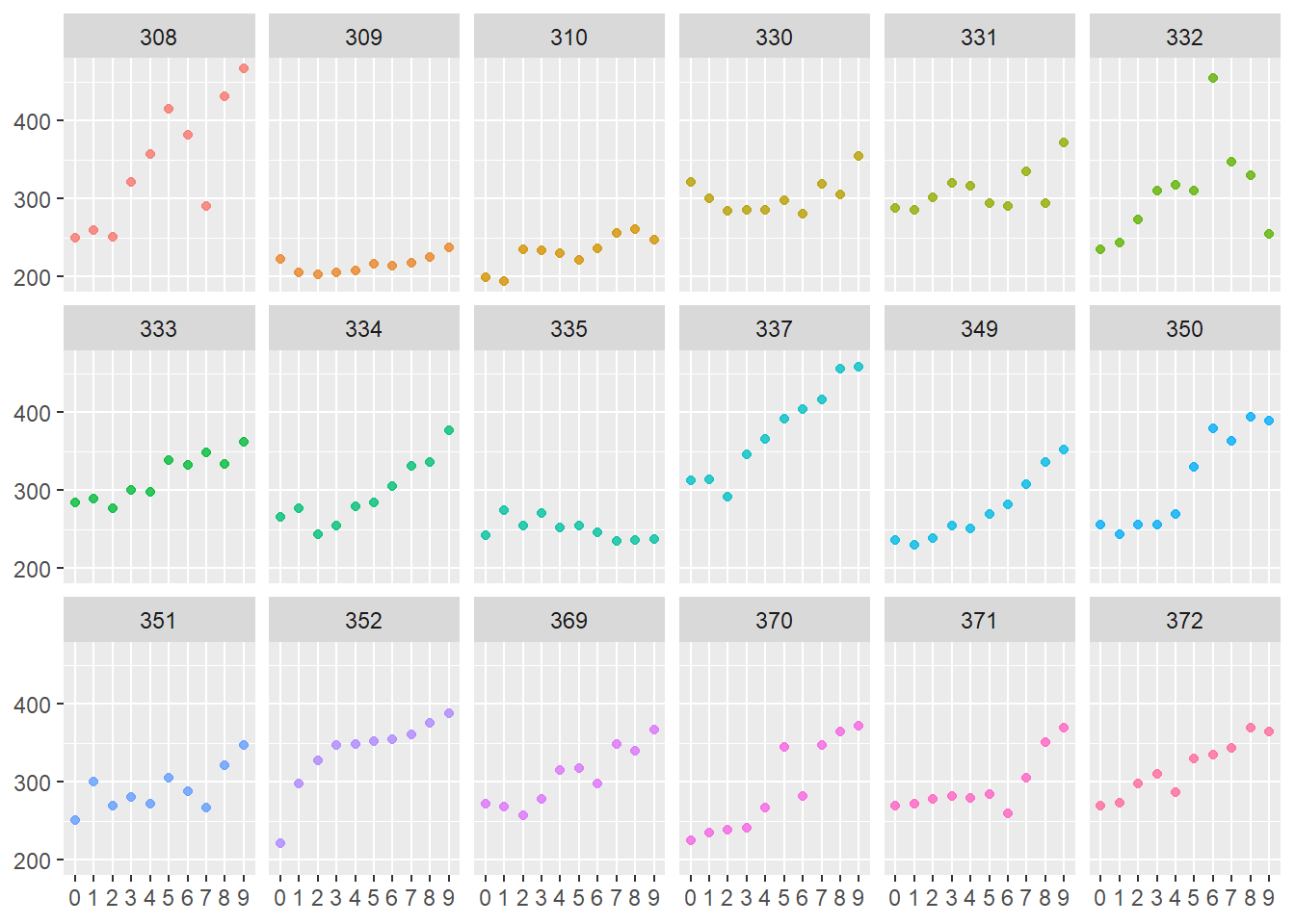
Further, the above plots appear to show an increase in reaction time with days of sleep deprivation that is somewhat linear in nature with slopes that differ significantly by Subject - a great scenario to investigate a multi-level model with a random intercept, btw.
tidyr::nest & purrr::map for Grouped Modeling
If you’re working with hierarchical data, it’s common to want build models among groups for comparison and review during EDA - e.g. what are the slopes of linear models fit to Reaction by Days for each Subject in the study?
This is the good motivation to employ tidyr::nest and purrr::map. I’ll walk through this procedure in two (2) steps:
- First I employ
nestafter grouping and thenmapto fit the model to eachSubject - Second I’ll extract the slopes from each model using
map_dbl, a flavor ofmap, and return it in a table.
# Step 1: group using `nest()` and fit a linear model
# to each subject and preview first 6 records:
sleepstudy %>%
  group_by(Subject) %>%
  nest() %>%
  mutate(models = map(data, ~lm(Reaction ~ Days , data = .x))) %>%
  head()
## # A tibble: 6 x 3
## # Groups: Subject [6]
## Subject data models
## <fct> <list> <list>
## 1 308 <tibble[,2] [10 x 2]> <lm>
## 2 309 <tibble[,2] [10 x 2]> <lm>
## 3 310 <tibble[,2] [10 x 2]> <lm>
## 4 330 <tibble[,2] [10 x 2]> <lm>
## 5 331 <tibble[,2] [10 x 2]> <lm>
## 6 332 <tibble[,2] [10 x 2]> <lm>Above, you’ll see two (2) new fields of type list in the resulting tibble including data - which includes the Reaction and Days for each Subject - and the models - the linear models fit for each.
Next, I show the entire code chunk including the mutate where I extract the slope of each linear fit from their respective model summaries. The result is a new parameter, slopes.
sleepstudy %>%
  # Step 1: group using `nest()`, fit a linear model
  # to each subject
  group_by(Subject) %>%
  nest() %>%
  mutate(models = map(data, ~lm(Reaction ~ Days , data = .x))) %>%
  # Step 2: extract the slope from each model
  # via model summary and preview first 6 records
  mutate(slopes = map_dbl(models,
                          ~summary(.x)$coefficients[[2]])) %>%
  head()
## # A tibble: 6 x 4
## # Groups: Subject [6]
## Subject data models slopes
## <fct> <list> <list> <dbl>
## 1 308 <tibble[,2] [10 x 2]> <lm> 21.8
## 2 309 <tibble[,2] [10 x 2]> <lm> 2.26
## 3 310 <tibble[,2] [10 x 2]> <lm> 6.11
## 4 330 <tibble[,2] [10 x 2]> <lm> 3.01
## 5 331 <tibble[,2] [10 x 2]> <lm> 5.27
## 6 332 <tibble[,2] [10 x 2]> <lm> 9.57The above pattern of tidyr::nest() followed by purrr::map() is extremely powerful when it comes to EDA for multilevel data and modeling review. For example, a similar code pattern can be created and extended to be used to simulate multilevel data for bootstrap estimation (i.e. sampling nested data ensures samples contain all their observations) - look out for this topic in a future post!
Other EDA Packages
I’ve merely scratched the surface when it comes to R’s EDA tools - for multilevel data or otherwise - so here are some other ones that I’ve found helpful in the past and present - tons of features to address the myriad of EDA tasks not covered in this post:
DataExplorer- several out-of-the box reports that look good with a lot of detailSmartEDA- a new-to-me package that provides tons of first-pass exploration options and presentation-worthy tablessummarytools- tons of output options with attractive crosstables
Here’s a quick look at the descr function from the summarytools package:
summarytools::descr(iris, stats = c("mean", "sd"),
                    transpose = TRUE, headings = FALSE) %>%
knitr::kable()| Mean | Std.Dev | |
|---|---|---|
| Petal.Length | 3.758000 | 1.7652982 |
| Petal.Width | 1.199333 | 0.7622377 |
| Sepal.Length | 5.843333 | 0.8280661 |
| Sepal.Width | 3.057333 | 0.4358663 |
Give these packages a look and you’re likely to find at least a few ways to ease your EDA procedures. That concludes today’s post so please take care, stay safe, and wear a mask!
References
Links
purrr, part of thetidyverseskimr, part of the rOpenSci project, a frictionless, pipeable approach to dealing with summary statistics- A
purrrtutorial by JBC
Data Considerations
Note that the lme4::sleepstudy data is an abridged version of the original data used for the analysis. The package version focuses only on the first 10 days - the sleep-deprivation part - of the study.