Mapping NYC’s 23K Trashcan Locations

The New York City Department of Sanitation (DSNY) - the largest department of its kind in the world - is responsible for the city’s garbage-collection operation. One component of this operation is the regular emptying of 23,000+ street-level trashcans - or as they call them: “litter baskets.”

DSNY offers up their geo-coded litter-basket inventory - refreshed monthly - through the NYC OpenData portal and in today’s post I’ll walk through how to create an interactive, 3D fly-over map of these litter-basket locations with the help of Mapbox’s Mapbox GL JS API in R.

Note: In order to follow along today’s post you will need to create a mapbox account and get yourself an access token, too.

DSNY Litter-Basket Data

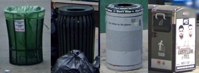
New York City-dwellers will recognize these four basket types found in the data:

Left-to-right: standard wire, high-end*, black-top, and solar-powered compacting baskets. Images via google street view

*high-end comes in several forms.

While each record is geo-coded, this particular data does not include the zip code of the basket location. To include that, I’ll use NYC zip code boundary shape files and the sf package to get the intersection between basket points and zip code boundaries.

pacman::p_load(here, tidyverse, glue, sf, mapboxer)
## pacman library: http://trinker.github.io/pacman
## Other libraries: RSocrata (to access NYC OpenData)

Zip code boundaries

First we download the shapefile for NYC zip codes and read it in using the sf package:

## download the file containing NYC's ZIP Code Boundaries
# dl_file <- tempfile()
# download.file(glue("https://data.cityofnewyork.us/download/", 
#                    "i8iw-xf4u/application%2Fzip"), dl_file)
# 
# ## unzip the file to the desired path
# unzip(dl_file, exdir=here(data_path, "nyc-zip-shapes", "zips"))

nyc_zips_geom <- st_read(here(data_path, "nyc-zip-shapes", "zips", 
                         "ZIP_CODE_040114.shp"), quiet = TRUE) %>% 
  select(ZIPCODE, PO_NAME, geometry)

DSNY basket inventory

I use RSocrata to read in the API resource and then use sf for the intersection between points and boundaries. Also included is some code for styling the map:

dsny_bin_url <- "https://data.cityofnewyork.us/8znf-7b2c"
bins <- RSocrata::read.socrata(dsny_bin_url) %>% 
  # 18 Baskets ('bins') have missing coords: BX (10), 
  # Q (6), BK (1), and SI (1) as of the publish date 
  filter(!is.na(stateplane_labelx)) %>%
  st_as_sf(coords = c("stateplane_labelx", "stateplane_labely"), 
           crs = st_crs(nyc_zips_geom))

# This intersection will provide us with the ZIP_CODE
# for each bin location tooltip.  
zipbins <- st_intersection(
  st_make_valid(bins), st_make_valid(nyc_zips_geom)
  ) %>%
  st_drop_geometry() %>% 
  st_as_sf(wkt = "point")

bname <- c("S" = "Standard Wire", "H" = "High-end", 
           "R" = "Black Top", "C" = "Compacting")

# DSNY Colors
bin_colorizer <- function(x) { 
  case_when( x == "S" ~ "#006749", x == "R" ~ "#1F2120", 
             x == "H" ~ "#2B8CFD", x == "C" ~ "#FBB039", 
             TRUE ~ "gray")
}

Here’s a look at the variable containing the data to be mapped, zipbins:

Rows: 24,702
Columns: 14
$ basketid             <int> 41260059, 41260057, 41260017, 4126…
$ baskettype           <chr> "H", "R", "H", "R", "H", "H", "S",…
$ direction            <chr> "SW", "SW", "NW", "SW", "NW", "SW"…
$ location_description <chr> "SW corner of SUTPHIN BLVD and FOC…
$ ownertype            <chr> "D", "D", "D", "D", "D", "D", "D",…
$ section              <chr> "QE126", "QE126", "QE126", "QE126"…
$ stateplane_snappedx  <dbl> 1041895, 1041416, 1041466, 1040899…
$ stateplane_snappedy  <dbl> 187226.9, 184748.9, 184818.8, 1848…
$ streetname1          <chr> "SUTPHIN BLVD", "ROCKAWAY BLVD", "…
$ streetname2          <chr> "FOCH BLVD", "145 ST", "145 ST", "…
$ objectid             <int> 20681, 20679, 20401, 18497, 16143,…
$ ZIPCODE              <chr> "11436", "11436", "11436", "11436"…
$ PO_NAME              <chr> "Jamaica", "Jamaica", "Jamaica", "…
$ point                <POINT> POINT (-73.79221 40.68026), POIN…

Mapboxer GL JS

The mapboxer package for R allows one to communicate with the Mapbox GLJS API. While it doesn’t offer easy access to the full functionality of the API, you can still achieve quite a lot with it. Below, I create the map showing all 23K+ litter-basket locations.

my_layer_id <- "baskets"                    # for live-filtering 
                                            # in the next section
basketmap <- zipbins %>% 
  mutate(basketcolor = bin_colorizer(baskettype), 
         baskettypename = ifelse(is.na(bname[baskettype]), 
                                 "Unknown", bname[baskettype])
  ) %>% 
  as_mapbox_source() %>% 
  mapboxer(                                 # basemap$Carto includes: 
    style = basemaps$Carto$positron,        # dark-matter, voyager, and
    center = c(-73.943362, 40.702051),      # positron.  6 mapbox styles
    zoom = 10, pitch = 40, width = "98%",   # are also offered
    max.zoom = 15
  ) %>%
  add_navigation_control() %>%
  add_circle_layer(
    circle_color = c("get", "basketcolor"),
    circle_blur = 1,
    circle_opacity = .8, 
    popup = paste0("<p>", 
                   "<div style='color:{{basketcolor}};margin:0 auto;'>",
                   paste0(rep("&#9644;",11), collapse = ""), 
                   "</div>",
                   "<b>{{baskettypename}} Basket</b><br>",
                   "{{PO_NAME}}, {{ZIPCODE}}<br>",
                   "Cross of: ",
                   "{{streetname1}} &<br>{{streetname2}}",
                   "<div style='color:{{basketcolor}}'>&#9671;</div>",
                   "</p>"), 
    id = my_layer_id
  )

DSNY Litter Basket Inventory Map

`r sprintf("%s", " ")`<svg width='10' height='10'><rect width='10' height='10' style='fill:#006749;stroke-width:1'/></svg> Standard Wire, High-end, Black Top, and Compacting

All data plotted is as of 2024-04-10. Click on points to see the zip code and other information about the baskets.

Native New Yorkers may recognize that some of the compacting baskets are clustered in high-traffic areas (e.g. Times Square). Some areas appear to have a higher density of baskets than others, too.

Live-filtering

Also great is the ability to add a query box to a map with mapboxer’s add_filter_control:

Using the query box inside the mapbox map

To achieve this I’ve made use of mapbox expressions for the filter argument. For example, changing the "H" to an "S" (capital S) in the query box in the below map immediately updates the view from “High-end” to “Standard Wire” baskets - give it a try for yourself:

basketmap %>%
  add_filter_control(
    my_layer_id,                            # Other Baskets:
    filter = list("==","baskettype", "H"),  # "R" = Black top
    pos = "top-left"                        # "C" = Solar-Powered 
  )                                         #       Compacting

While the query box doesn’t provide what I’d call an “end-user experience,” it’s a very helpful feature for quick prototyping and EDA for the technically-inclined data professional.

Conclusion

When you need to plot tens of thousands of points on a map, standard analysis tools can get overwhelmed and can become sluggish to the point of being unusable. Add a requirement for interactivity to the mix, and the number of solutions available to your average data professional becomes even smaller.

Mapbox GL JS met this challenge without skipping a beat while only hinting at the full suite of feature-offerings. Still, rather than overwhelm you, I’ll end today’s post here - take care!