Translating Tract-Level ACS Data to NYPD Precincts

In this posts I’m going to demonstrate how to get NYC census data at the tract level to estimate census data at the NYPD-precinct level.

There are 77 NYPD precincts serving five boroughs of NYC and each precinct contains multiple census tracts. To get the census-level demographics on a per-precinct level, I’ll need a way to aggregate the tract data into precincts - let’s get started!

library(sf)            # getting intersectional geographies
library(tidyverse)     # wrangling
library(tidycensus)    # nyc shape files and deomgraphic data
census_api_key("YOUR_CENSUS_API_KEY", install = T, overwrite = T)
library(tigris)        # area_water function
library(tmap)          # visualizations
library(here)          # for directory navigation # new 2020-10-20

note: The code below has been updated as of 2020-07-04 to conform to some library updates and R updates.

Getting the Precinct Map

First I pull in the geojson data from the NYC City Planning website for “Police Precincts (Clipped to Shoreline)”:

# This URL REGULARLY changes - I'd check with the link above 
# to ensure you're getting an up-to-date file
prcts_url <- paste0("https://services5.arcgis.com/GfwWNkhOj9bNBqoJ/arcgis", 
                    "/rest/services/NYC_Police_Precincts/FeatureServer/0/", 
                    "query?where=1=1&outFields=*&outSR=4326&f=geojson")
precinct_map <- read_sf(prcts_url) %>%
  st_transform(2263)

# add X, Y coordinates for precinct labels
precinct_map <- cbind(precinct_map, 
                      st_coordinates(st_centroid(precinct_map, 
                                                 of_largest_polygon =T)))

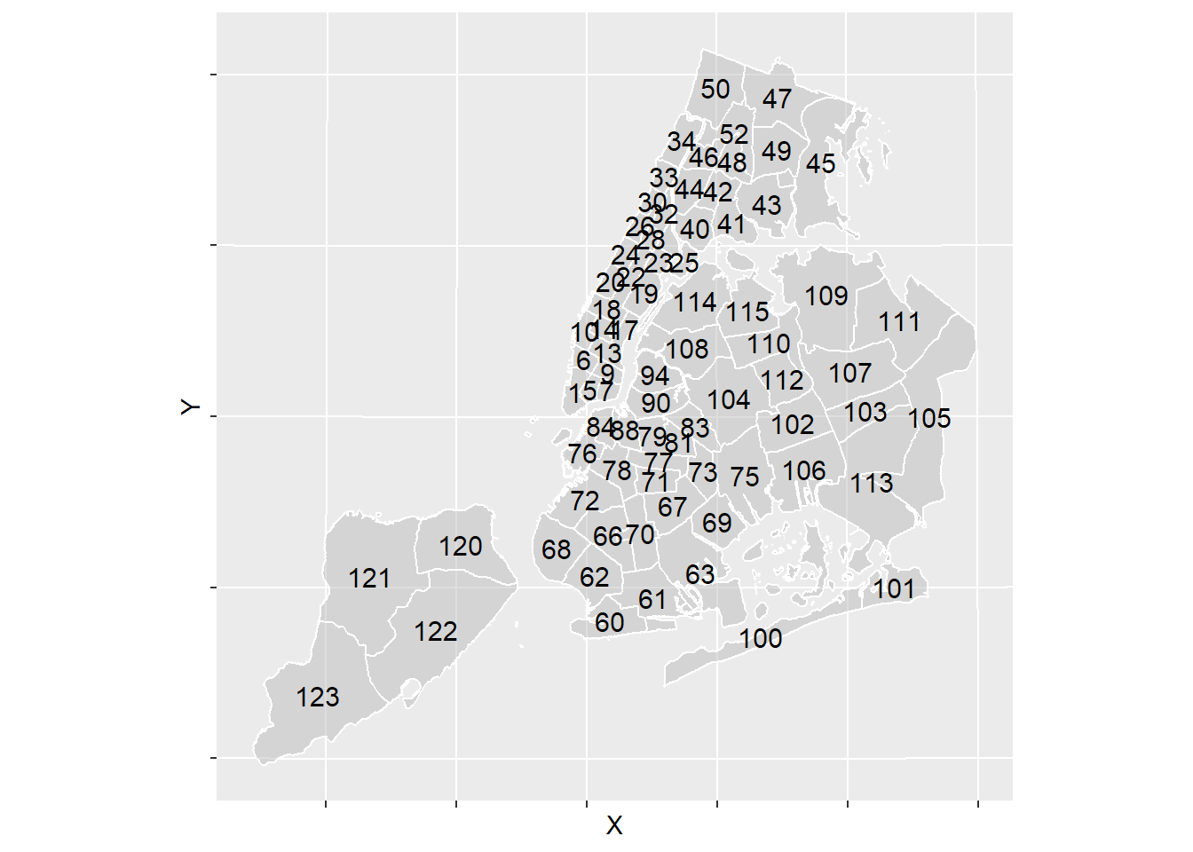
Let’s take a look:

ggplot()+
  geom_sf(data = precinct_map[, "Precinct"], alpha = .5, 
          color = "white", fill = "gray")+
  geom_text(data = precinct_map, aes(X, Y, label = Precinct), 
            size = 4, color = "black" )+
  theme(legend.position = "none", 
        axis.text = element_blank())

NYC residents may recognize how the numbering schema can tell you what borough a precinct resides.

Intersecting the Census Map with the Precinct Map

Getting the ACS Map at the Tract Level

Since precincts cover many census tracts, I will use the area of each precinct that intersects with tract-level areas to calculate the ACS estimates at a per-precinct level.

First I get the 2016 ACS data via tidycensus along with the geometries of the census tracts. Then I clip the water area from the shape files using the area_water function from the tigris package - this is done to ensure that the areas within the census map tracts are closely aligned with the area of the water-clipped police precinct boundaries - see my last post for a demonstration of how to obtain census data with shape files via tidycensus.

Overlaying Census Map with Precinct Map

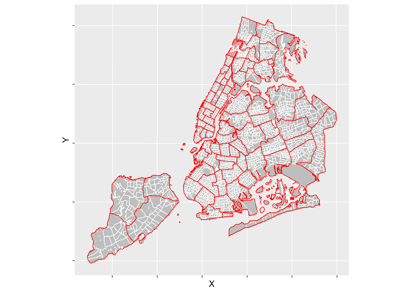
Next I map the water-clipped census tract map from tidycensus with an overlay of the NYPD precinct map. Here we can see just how many census tracts fit in each precinct. I’ve highlighted the 34th precinct as we’ll be focusing on that precinct for the remainder of the post to keep things digestible.

p1 <- ggplot()+
  geom_sf(data = nyc_census[nyc_census$variable=="ToPop","GEOID"], 
          color = "white", fill = "gray")+
  geom_sf(data = precinct_map[, "Precinct"], color = "red", fill = "NA")+ 
  geom_sf(data = precinct_map %>% filter(Precinct==34),
          color = "red", fill = "red", alpha = .3)+
  geom_text(data = precinct_map %>% filter(Precinct==34), 
            aes(X, Y, label = Precinct), 
            fontface = "bold",
            color = "white") +
  theme(axis.text = element_blank())

p1

Obtaining Precinct/Census-Tract Intersections

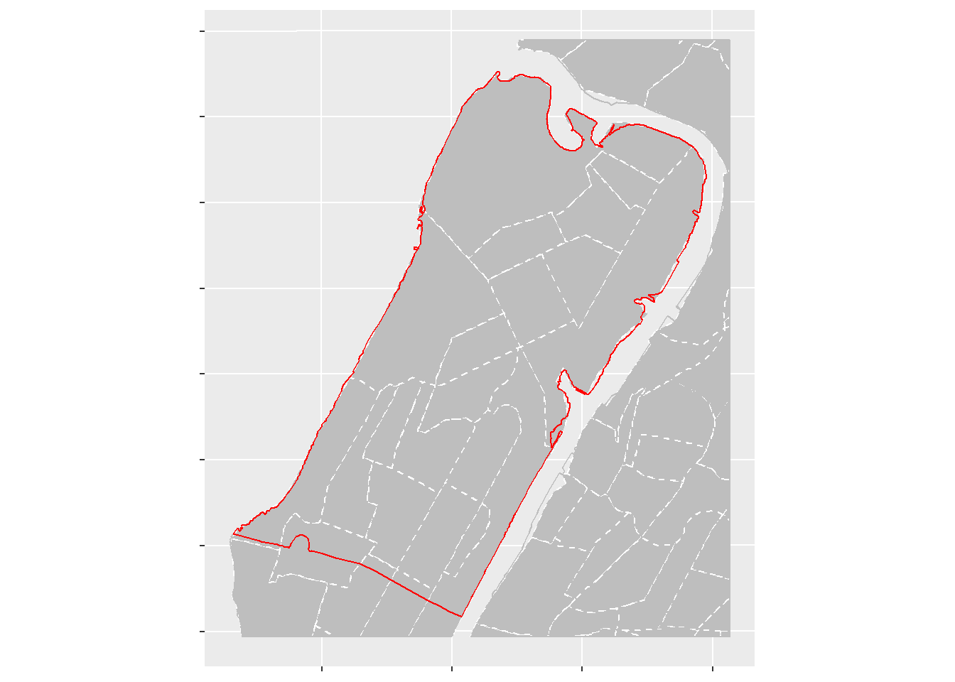
Now onto using the intersections of polygons to get the census tract data into the 34th precinct. Below we see a zoomed-in view of the 34th precinct. The census tract boundaries are outlined in gray dashed lines with the outline of the precinct in red.

Notice how some census tracts in the southern part of the 34th are clipped by the boundary of the precinct and how the precinct map doesn’t perfectly cover census map’s perimeter. This will certainly impact the estimations but I’ll address that shortly.

To get the intersection areas I use sf’s st_area function to obtain the census tract areas and then compute the percentage of those areas that fall within the precinct using st_intersection.

nyc_census <- nyc_census %>% 
  mutate(area = st_area(.) %>% as.numeric())

mini_intersect <- st_intersection(st_make_valid(
  precinct_map[precinct_map$Precinct==34, 
               c("Precinct")]),nyc_census) %>% 
  mutate(intersect_area = st_area(.) %>% as.numeric(), 
         intersect_wt = intersect_area/area, 
         est_wt = estimate * intersect_wt)

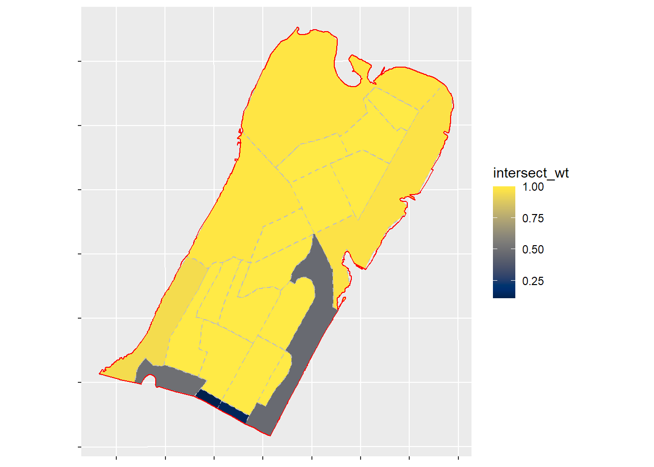
And here’s the plot of mini_intersect:

As shown above, the tracts that are totally within the bounds of the 34th precinct are showing 100% (or close to 100%) intersect weights while tracts that are cut along the precinct boundaries do not. There are some slight under-estimates for tracts along the water-line but this marginal error was expected and can be mitigated slightly via st_buffer from the sf package as we’ll soon see.

Here’s a preview of census data intersected with the 34 precinct that includes the intersection weight column (intersect_wt):

mini_intersect %>% glimpse()

Rows: 220
Columns: 10
$ Precinct       <int> 34, 34, 34, 34, 34, 34, 34, 34, 34, 34, 34, 34, 34, 34,~
$ GEOID          <chr> "36061030700", "36061026100", "36061028100", "360610273~
$ NAME           <chr> "Census Tract 307, New York County, New York", "Census ~
$ variable       <chr> "AmIAN", "AmIAN", "AmIAN", "AmIAN", "AmIAN", "AmIAN", "~
$ estimate       <dbl> 0, 0, 0, 0, 0, 0, 0, 0, 22, 0, 0, 0, 0, 0, 0, 0, 0, 0, ~
$ area           <dbl> 908178.9, 1681544.9, 1014226.9, 1904592.7, 2076418.3, 1~
$ geometry       <GEOMETRY [US_survey_foot]> POLYGON ((1007743 256837.6,..., P~
$ intersect_area <dbl> 908178.9, 232343.1, 1014226.9, 1904592.7, 2076418.3, 16~
$ intersect_wt   <dbl> 1.0000000, 0.1381724, 1.0000000, 1.0000000, 1.0000000, ~
$ est_wt         <dbl> 0.0000000, 0.0000000, 0.0000000, 0.0000000, 0.0000000, ~

Depending on the ACS statistic you’ve got in your tidycensus data, you will need to consider how you will aggregate. You can sum the population estimates that are multiplied by the intersection weight or you can use the weighted.mean function if your ACS data contains something like median income.

From this point, getting the remainder of the precinct stats follows a similar workflow:

Get intersection areas of each census tract within a precinct
Calculate the weights (i.e. the percentage of each tract area that falls within precinct boundary) by dividing each tract area that intersects a precinct area by the total tract.
Multiply ACS estimate by weight and aggregate by precinct (sum or weighted.mean).

To mitigate the water-line clipping error, I’ll use st_buffer on the precinct map to very-marginally increase the perimeter of the precinct boundary to capture clipped census tract areas.

Here is a preview of the racial breakdown of each precinct after I completed the steps outlined above:

nyc_precincts %>% spread(variable, est_wt) %>% glimpse(width = 78)

Rows: 77
Columns: 13
$ Precinct <int> 1, 5, 6, 7, 9, 10, 13, 14, 17, 18, 19, 20, 22, 23, 24, 25, ~
$ geometry <GEOMETRY [US_survey_foot]> MULTIPOLYGON (((971153.8 19..., POLYG~
$ boro     <dbl> 1, 1, 1, 1, 1, 1, 1, 1, 1, 1, 1, 1, 1, 1, 1, 1, 1, 1, 1, 1,~
$ AmIAN    <dbl> 3.741962e+01, 8.290712e+01, 1.404972e+02, 1.480272e+02, 9.3~
$ Asian    <dbl> 11576.36206, 28557.81050, 5252.47747, 18339.33586, 10209.76~
$ AsianPI  <dbl> 11581.20865, 28565.65666, 5256.48994, 18339.85926, 10299.76~
$ Black    <dbl> 1766.48558, 2496.31012, 1131.16454, 4889.36049, 5707.74607,~
$ LatBl    <dbl> 90.66727, 953.90428, 65.88356, 731.49897, 607.54032, 568.85~
$ LatWh    <dbl> 3947.42376, 3319.80088, 2616.87710, 6648.24281, 7230.24475,~
$ NaHPI    <dbl> 4.846595e+00, 7.846161e+00, 4.012467e+00, 5.233997e-01, 8.9~
$ Other    <dbl> 3885.59356, 3822.91050, 2299.35648, 12042.48100, 11613.4656~
$ ToPop    <dbl> 69519.0038, 51372.9958, 60599.8905, 55460.6035, 75857.2328,~
$ White    <dbl> 48210.2053, 12131.5062, 49089.6217, 12661.1338, 40305.2642,~

And to show that the intersection method provides a decent estimation, here is the difference in NYC population from the original census data and the intersected precinct data. As shown in the comments, adding different values to st_buffer for the precinct map produced population estimates that varied from the original census data. I went with st_buffer(3) as it provided the closest population estimate without going over among the values I tried.

cropped <- nyc_precincts[nyc_precincts$variable=="ToPop","est_wt"]$est_wt %>% sum()
original <- nyc_census[nyc_census$variable=="ToPop",]$estimate %>% sum()

cropped/original * 100 #   99.7871 without buffer

[1] 99.9252

                       #   99.8779 with nyc_precincts %>% st_buffer(2)
                       #   99.9224 with                   st_buffer(3) ***
                       #  100.0103 with                   st_buffer(5)
                       #  100.4348 with                   st_buffer(15)
                       #  100.8437 with                   st_buffer(25)
                       #  101.8398 with                   st_buffer(50)

99.93% is more than enough accuracy to confidently make a choropleth of ACS population by NYPD precinct - I’m missing less than 7K residents from a population of almost 8.5M:

Closing Remarks