Web Scraping for Public Health Data
Part of the new normal for many data analytics professionals is being able to obtain Covid-19 data by geographic location. To address this need, today’s post is going to walk through how to scrape the repo for the NYC Department of Health and Mental Hygiene using the flexible rvest library to to create a time-series of positive cases by NYC zip code.
The Target Data
As a resident of NYC, the former epicenter of the outbreak, I’ve been keen on getting some time series data on Covid 19 to see how things are coming along.
To that end, I’ve been pulling NYC Health’s coronavirus-data since they began sharing it and I’ve seen how it’s evolved over time. E.g. at first, tests-by-zcta.csv was the only zip-code-focused and later they added data-by-modzcta.csv; essentially the same data but with different field names and additional columns.
In order to create the most comprehensive dataset with the longest time-frame available, I would have to combine these files over time referencing the historical commits to their respective repos.
Web Scraping
library(tidyverse) # data manipulation
library(glue) # string manipulation
library(rvest) # webscraping
library(xml2) # dependency for rvest
library(tsibble) # time-series aggregation
## Other libraries in use but not downloaded here:
# plyr::rbind.fill() # stacking dfs with only some matching columns
# tidyr::fill() # for days when data isn't collected
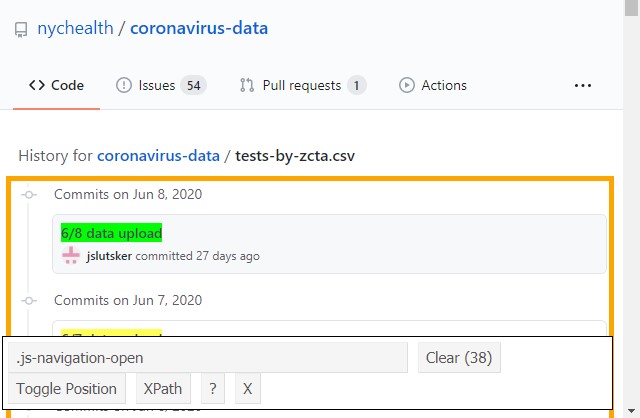
# lubridate:: # all things date formattingA key component of web-scrapping is being able to identify different parts of a webpage using the DOM (Document Object Model). I do this with the help of the SelectorGadget for Chrome, going to the web page of interest, enabling SelectorGadget, and clicking on the components of interest. Below I’ve included a screen cap of the ".js-navigation-open" component that contains the link to the historical files.
 After a few minutes playing around, I was able to find the page elements containing the data I needed. This stuff isn’t straight-forward so it’s probably best to start with the example given in the
 rvest documentation: it’s very good and worth a read if you want to understand what’s going on under the hood before diving in.
The first step will be to obtain the URLs to all historical files and the second step will be to download the data stored in each of those URLs.
The File URLs
base_url = "https://raw.githubusercontent.com/nychealth/coronavirus-data/"

historical_urls_pg1 <- glue("https://github.com/nychealth/coronavirus-data/",
                            "commits/master/tests-by-zcta.csv")

second_page_url <- function(url){
  # expects the URL pointing to the file's commit history on git
  # pull the last button from the page (Older)
  pg <- xml2::read_html(url)
  paginate <- rvest::html_nodes(pg, ".paginate-container , .BtnGroup-item")
  rvest::html_attr(paginate[[length(paginate)]], "href")
}

# it would be better to make this such that it can handle any page length.
historical_urls_pg2 <- second_page_url(historical_urls_pg1)

historical_urls_new <- glue("https://github.com/nychealth/coronavirus-data/",
                            "commits/master/data-by-modzcta.csv")

c19_url <- function(git_code, closer = "tests-by-zcta.csv"){
    base_url = "https://raw.githubusercontent.com/nychealth/coronavirus-data/"
  glue::glue(base_url, git_code, "/", closer)
}

get_historical_covid <- function(url){
  # scrapes github for previously committed versions over time
  # places the URLs and commit dates into a df
  pg <- xml2::read_html(url)
  date_nodes <- rvest::html_nodes(pg, ".no-wrap")
  dates_raw <- rvest::html_nodes(pg, "relative-time") %>% as.list()

  file_urls <- rvest::html_nodes(pg, ".js-navigation-open")
  rel_urls <- rvest::html_attr(file_urls, "href")
  rel_urls <- rel_urls[lapply(rel_urls,nchar)>0] %>% as.list()

  # dates of historical files (commit datetime)
  dates <- substr(dates_raw, 26, 44) #%>% length()
  # url codes for historical files
  files <- substr(rel_urls,36, 75)

  if (length(dates) == length(files)){
    return(tibble::tibble(commit_date = dates, git_code = files))
  }else{
    print("broken!")
  }
}
This will allow me to obtain a combined list of URLs for each of the files. I then loop through the list and download a tibble for each historical version of the files.
Note: If this were many, many sources and multiple pages of history, I would probably set this up differently:
url <- c(historical_urls_pg1, historical_urls_pg2)

# combine the pages of the URLS for test-by-zcta...
df <- rbind(get_historical_covid(url[[1]]),
            get_historical_covid(url[[2]])) %>%
  mutate(source = "tests-by-zcta.csv")

# obtain historical urls for data-by-modacta.csv
dff <- get_historical_covid(historical_urls_new) %>%
  mutate(source = "data-by-modzcta.csv")

all_urls <- rbind(df, dff) %>%
  mutate(commit_date = lubridate::ymd_hms(commit_date)) %>%
  arrange(commit_date) %>%
  mutate(file_url = glue::glue("{base_url}{git_code}/{source}"))

read_csv_check <- function(f, c_date, src, ...) {
  # for reading the GITHUB url, adding details & src.
  tryCatch({vroom::vroom(f) %>%
             select_all(tolower) %>%
             mutate(commit_date = c_date,
                    source = src)},
           error = function(c) {
    print(paste0(c$message, " (in ", f, ")"))
    invisible()
  })
}
Here’s a preview of the all_urls variable and it’s contents:
## Rows: 102
## Columns: 4
## $ commit_date <dttm> 2020-04-01 16:35:56, 2020-04-03 22:56~
## $ git_code    <chr> "097cbd70aa00eb635b17b177bc4546b2fce21~
## $ source      <chr> "tests-by-zcta.csv", "tests-by-zcta.cs~
## $ file_url    <glue> "https://raw.githubusercontent.com/ny~
The Files
The below chunk does the actual URL-reading but I’ve suppressed the output because it’s a bit verbose.
covid_dfs <- list()
covid <- tibble()

## Create a long list dfs from the URLs (skip the 404s)
for (i in seq_along(all_urls$git_code)){
  temp <- read_csv_check(f = all_urls[i,]$file_url %>% as.character(),
                         c_date = all_urls$commit_date[[i]],
                         src = all_urls$source[[i]])
  ## if you're intereted in seeing it work
  #print(glue::glue("File {temp$source %>% unique()}"))
  #print(glue::glue("Commit Date {temp$commit_date %>% unique()}"))
  #print(glue::glue("Columns {temp %>% colnames()}"))
  covid_dfs <- covid_dfs %>%
    append(list(temp))
}
Above, covid_dfs is a list of tibbles, each containing a historical version of the files, here’s a look at it:
## Rows: 178
## Columns: 5
## $ modzcta     <dbl> NA, 10001, 10002, 10003, 10004, 10005,~
## $ positive    <dbl> 32, 113, 250, 161, 16, 25, 6, 26, 181,~
## $ total       <dbl> 36, 265, 542, 379, 38, 81, 24, 67, 450~
## $ commit_date <dttm> 2020-04-01 16:35:56, 2020-04-01 16:35~
## $ source      <chr> "tests-by-zcta.csv", "tests-by-zcta.cs~
Data Cleanup
Metadata Prep
First step is creating a mapping table containing zip code, neighborhood names, and borough fields. It appears they started using a consistent naming format after 2020-06-27.
c_date_func <- function(a_date){substr(as.character(a_date),1,10)}

neighborhood <- covid_dfs %>%
  plyr::rbind.fill() %>%
  as_tibble() %>%
  dplyr::select(modified_zcta, neighborhood_name,
                borough_group, commit_date) %>%
  na.omit() %>%
  # I filter on the 2020-06-27 as this appears to be the latest
  # neighborhood_name version
  filter(commit_date > as.Date("2020-06-27")) %>%
  mutate(modified_zcta = as.character(modified_zcta)) %>%
  distinct() %>%
  dplyr::select(zip_code = modified_zcta,
                neighborhood_name, borough_group)
And here’s a preview of the cleaned up neighborhood variable:
## Rows: 5,841
## Columns: 3
## $ zip_code          <chr> "10001", "10002", "10003", "1000~
## $ neighborhood_name <chr> "Chelsea/NoMad/West Chelsea", "C~
## $ borough_group     <chr> "Manhattan", "Manhattan", "Manha~
Core Data Prep
Next I create the core data. I have narrowed the example to include the date, count of positive tests recorded, and the zip code. There is a bit of overlap between the files and I take the median if more than one measure is encountered per day.
Since this data is a time-series, I employ the tsibble package as it’s got utilities to deal with gaps in the records.
# covid time series = c_ts containing
# - f_date: commit date of the file
# - zip_code:
# - covid_case_count = "positive tests recorded"
covid_ts <- covid_dfs %>%
  plyr::rbind.fill() %>%
  as_tibble() %>%
  mutate(modified_zcta = ifelse(is.na(modified_zcta),
                                modzcta, modified_zcta),
         covid_case_count = ifelse(is.na(covid_case_count),
                                   as.numeric(positive),
                                   as.numeric(covid_case_count)),
         commit_date = as.POSIXct(commit_date),
         f_date = c_date_func(commit_date),
         modified_zcta = ifelse(modified_zcta == 99999,
                                NA_real_, modified_zcta)
         ) %>%
  dplyr::select(source:f_date) %>%
  dplyr::distinct() %>%
  dplyr::group_by(f_date, zip_code = modified_zcta) %>%
  ## Create the time series of covid case count (positive covid tests)
  ## by combining sources & taking median where there's overlap
  dplyr::summarise(covid_case_count = mean(covid_case_count, na.rm = T),
                   .groups = "drop") %>%
  mutate(f_date = lubridate::ymd(f_date),
         zip_code = as.character(zip_code)) %>%
  left_join(neighborhood, by="zip_code", all.x = T) %>%
  distinct()

# These dates appear to show data corrections:
odd_entries <- c(as.Date("2020-04-26"), as.Date("2020-05-23"),
                 as.Date("2020-09-26"), as.Date("2020-09-27"),
                 as.Date("2020-09-28"))

covid_ts <- as_tsibble(covid_ts,
                       key = c(zip_code, neighborhood_name, borough_group),
                       index = f_date) %>%
  filter(!(f_date %in% odd_entries))
And here’s a preview of first-pass view of the covid_ts data that I’ve created:
## Rows: 16,526
## Columns: 5
## Key: zip_code, neighborhood_name, borough_group [179]
## $ f_date            <date> 2020-04-01, 2020-04-03, 2020-04~
## $ zip_code          <chr> "10001", "10001", "10001", "1000~
## $ covid_case_count  <dbl> 113, 136, 146, 158, 170, 178, 19~
## $ neighborhood_name <chr> "Chelsea/NoMad/West Chelsea", "C~
## $ borough_group     <chr> "Manhattan", "Manhattan", "Manha~
Gaps in Temporal Data
Whenever you receive time-series data it’s a good idea to check for gaps. Observations that may have been missed one day but return the next. Thankfully, the tsibble library contains several helpful utilities for looking over temporal data.
The first function is count_gaps that takes a tsibble and returns the elements of the index (zip_code in this example) along with the .from and .to dates in which there is missing data. Here’s a glimpse of that data:
## Rows: 1,778
## Columns: 6
## $ zip_code          <chr> "10001", "10001", "10001", "1000~
## $ neighborhood_name <chr> "Chelsea/NoMad/West Chelsea", "C~
## $ borough_group     <chr> "Manhattan", "Manhattan", "Manha~
## $ .from             <date> 2020-04-02, 2020-04-06, 2020-04~
## $ .to               <date> 2020-04-02, 2020-04-06, 2020-04~
## $ .n                <int> 1, 1, 1, 1, 1, 1, 1, 1, 120, 103~
From the above we can see that zip code 10001, for example, is missing data on 2020-04-02, 2020-04-06, etc. We can fill those gaps with NAs using the fill_gaps function:
covid_ts %>%
  fill_gaps(.full = start()) %>%
  head()
## # A tsibble: 6 x 5 [1D]
## # Key: zip_code, neighborhood_name, borough_group [1]
## f_date zip_code covid_case_count neighborhood_name borough_group
## <date> <chr> <dbl> <chr> <chr>
## 1 2020-04-01 10001 113 Chelsea/NoMad/West Chelsea Manhattan
## 2 2020-04-02 10001 NA Chelsea/NoMad/West Chelsea Manhattan
## 3 2020-04-03 10001 136 Chelsea/NoMad/West Chelsea Manhattan
## 4 2020-04-04 10001 146 Chelsea/NoMad/West Chelsea Manhattan
## 5 2020-04-05 10001 158 Chelsea/NoMad/West Chelsea Manhattan
## 6 2020-04-06 10001 NA Chelsea/NoMad/West Chelsea ManhattanIn time series analysis, it’s common to replace NA’s with their previous observation for each origin, which I do here using tidyr::fill:
covid_ts %>%
  fill_gaps(.full = start()) %>%
  tidyr::fill(covid_case_count, .direction = "down") %>%
  head()
## # A tsibble: 6 x 5 [1D]
## # Key: zip_code, neighborhood_name, borough_group [1]
## f_date zip_code covid_case_count neighborhood_name borough_group
## <date> <chr> <dbl> <chr> <chr>
## 1 2020-04-01 10001 113 Chelsea/NoMad/West Chelsea Manhattan
## 2 2020-04-02 10001 113 Chelsea/NoMad/West Chelsea Manhattan
## 3 2020-04-03 10001 136 Chelsea/NoMad/West Chelsea Manhattan
## 4 2020-04-04 10001 146 Chelsea/NoMad/West Chelsea Manhattan
## 5 2020-04-05 10001 158 Chelsea/NoMad/West Chelsea Manhattan
## 6 2020-04-06 10001 158 Chelsea/NoMad/West Chelsea ManhattanNote that we’ve filled in the missing dates with the prior day’s value. Finally, I put all the steps together and filter out a few zip codes that appear to have been included in error as they’re only included in a single day of data 5/23/2020:
Visualize the Data
Finally, to complete the example, I plot the sum of the daily differences for a random zip code, 10040
my_plot <- covid_ts %>%
  arrange(zip_code, f_date) %>%
  mutate(f_month = lubridate::month(f_date, label=T),
         f_week = lubridate::week(f_date),
         f_day = lubridate::day(f_date),
         f_wday = lubridate::wday(f_date, label = T),
         dailydiff = difference(covid_case_count,lag = 1),
         diff_7day_ma = slider::slide(dailydiff, mean,
                                  na.rm = TRUE, .size = 7)) %>%
  filter(f_date > covid_ts$f_date %>% min()+7) %>%
  group_by(f_month, f_day, borough_group) %>%
  summarise(SumOfDailyDiff = sum(dailydiff)) %>%
  na.omit() %>%
  filter(f_date < as.Date("2020-06-7")) %>%
  ggplot(aes(x = f_date, y = SumOfDailyDiff))+
    geom_line()+
  facet_wrap(~borough_group)+
  labs(title = "Sum, Daily Differences in C19 Case Count;10040")+
  theme(axis.title.x = element_blank(),
        axis.title.y = element_blank())

plotly::ggplotly(my_plot)
As of the latest available data for this post, the plots paint a promising picture but I am going to remain cautiously optimistic given the recent spikes showing in the Bronx and Brooklyn. The weather’s been really nice, too, which is a blessing and curse in times like these.
Please stay safe out there and take care!