Multiple Linear Regression Modelling; Money Ball
In this post I will pre-process, explore, transform, and model data from baseball team seasons from 1871-2006 inclusive (stats adjusted to match 162-game season). Feature additions and transformations can improve the predictive power of created models and in this post I’ll employ a Box-Cox transformation to acheive this.
The goal is to create a model that can predict baseball team wins based on the performance metrics captured in the training dataset moneyball-training-data.csv and then review the predictive quality by running the model with moneyball-evaluation-data.csv the testing dataset.
Libraries in use:
library(stargazer)
library(tidyverse)
library(RCurl)
library(MASS)
Data Exploration
High-level Findings
- There are ~2300 observations with 16 variables included
- Five of the variables have a number of missing values
- Two of the variables have outliers
- Multicollinearity present in seven variables
- Untransformed (raw) data is not highly correlated with response
# read in data.
mb_train <- paste0("https://raw.githubusercontent.com/jbrnbrg/",
                   "msda-datasets/master/moneyball-training-data.csv")
mb_eval <- paste0("https://raw.githubusercontent.com/jbrnbrg/",
                   "msda-datasets/master/moneyball-evaluation-data.csv")

bsb_train_raw <- read_csv(mb_train)
##
## -- Column specification --------------------------------------------------------
## cols(
## INDEX = col_double(),
## TARGET_WINS = col_double(),
## TEAM_BATTING_H = col_double(),
## TEAM_BATTING_2B = col_double(),
## TEAM_BATTING_3B = col_double(),
## TEAM_BATTING_HR = col_double(),
## TEAM_BATTING_BB = col_double(),
## TEAM_BATTING_SO = col_double(),
## TEAM_BASERUN_SB = col_double(),
## TEAM_BASERUN_CS = col_double(),
## TEAM_BATTING_HBP = col_double(),
## TEAM_PITCHING_H = col_double(),
## TEAM_PITCHING_HR = col_double(),
## TEAM_PITCHING_BB = col_double(),
## TEAM_PITCHING_SO = col_double(),
## TEAM_FIELDING_E = col_double(),
## TEAM_FIELDING_DP = col_double()
## )mini_tbl<-psych::describe(bsb_train_raw[,-1], IQR=T)[,c(1:5,8:10,12,14)]
bsb_train <- data.table::setnames(bsb_train_raw,
tolower(names(bsb_train_raw[1:17])))
bsb_train[is.na(bsb_train)] <- 0 # used for simple plots - not used for model fitting
# see data preperation section for more details.
col_name_updater <- function(x, text_to_updt, replc_text){
colnames(x) = gsub(text_to_updt, replc_text, colnames(x))
return(x)
}
# shorten and clean colnames
c1 <- col_name_updater(bsb_train, "batting", "bat")
c2 <- col_name_updater(c1, "pitching", "pitch")
c3 <- col_name_updater(c2, "fielding", "field")
c4 <- col_name_updater(c3, "baserun", "baser")
bsb_data <- col_name_updater(c4, "team", "t")
rm(c1,c2,c3, c4)
c1 <- col_name_updater(bsb_train_raw, "batting", "bat")
c2 <- col_name_updater(c1, "pitching", "pitch")
c3 <- col_name_updater(c2, "fielding", "field")
c4 <- col_name_updater(c3, "baserun", "baser")
bsb_train_raw <- col_name_updater(c4, "team", "t")
rm(c1,c2,c3, c4)Findings Detail
The below investigation was completed prior to model-fitting in order to get a sense for the density and quality of the training data set and to preview what types of actions may need to be taken in the model-fitting steps.
Summary Statistics:
| vars | n | mean | sd | median | min | max | range | kurtosis | IQR | |
|---|---|---|---|---|---|---|---|---|---|---|
| TARGET_WINS | 1 | 2276 | 80.79 | 15.75 | 82.0 | 0 | 146 | 146 | 1.03 | 21.00 |
| TEAM_BATTING_H | 2 | 2276 | 1469.27 | 144.59 | 1454.0 | 891 | 2554 | 1663 | 7.28 | 154.25 |
| TEAM_BATTING_2B | 3 | 2276 | 241.25 | 46.80 | 238.0 | 69 | 458 | 389 | 0.01 | 65.00 |
| TEAM_BATTING_3B | 4 | 2276 | 55.25 | 27.94 | 47.0 | 0 | 223 | 223 | 1.50 | 38.00 |
| TEAM_BATTING_HR | 5 | 2276 | 99.61 | 60.55 | 102.0 | 0 | 264 | 264 | -0.96 | 105.00 |
| TEAM_BATTING_BB | 6 | 2276 | 501.56 | 122.67 | 512.0 | 0 | 878 | 878 | 2.18 | 129.00 |
| TEAM_BATTING_SO | 7 | 2174 | 735.61 | 248.53 | 750.0 | 0 | 1399 | 1399 | -0.32 | 382.00 |
| TEAM_BASERUN_SB | 8 | 2145 | 124.76 | 87.79 | 101.0 | 0 | 697 | 697 | 5.49 | 90.00 |
| TEAM_BASERUN_CS | 9 | 1504 | 52.80 | 22.96 | 49.0 | 0 | 201 | 201 | 7.62 | 24.00 |
| TEAM_BATTING_HBP | 10 | 191 | 59.36 | 12.97 | 58.0 | 29 | 95 | 66 | -0.11 | 16.50 |
| TEAM_PITCHING_H | 11 | 2276 | 1779.21 | 1406.84 | 1518.0 | 1137 | 30132 | 28995 | 141.84 | 263.50 |
| TEAM_PITCHING_HR | 12 | 2276 | 105.70 | 61.30 | 107.0 | 0 | 343 | 343 | -0.60 | 100.00 |
| TEAM_PITCHING_BB | 13 | 2276 | 553.01 | 166.36 | 536.5 | 0 | 3645 | 3645 | 96.97 | 135.00 |
| TEAM_PITCHING_SO | 14 | 2174 | 817.73 | 553.09 | 813.5 | 0 | 19278 | 19278 | 671.19 | 353.00 |
| TEAM_FIELDING_E | 15 | 2276 | 246.48 | 227.77 | 159.0 | 65 | 1898 | 1833 | 10.97 | 122.25 |
| TEAM_FIELDING_DP | 16 | 1990 | 146.39 | 26.23 | 149.0 | 52 | 228 | 176 | 0.18 | 33.00 |
Missing Values:
Review of the NA’s (see column n, Table1) revealed the following sparse variables. The value after the variable name represents the number of missing values followed % density on 2,276 records available in most (11 of 16) variables:
TEAM_BATTING_HBP: 2085: 8%TEAM_BASERUN_CS: 772: 66%TEAM_FIELDING_DP: 286: 87%TEAM_PITCHING_SO: 102: 96%TEAM_BATTING_SO: 102: 96%
Outliers:
Below, a preview of each variable in the data using box plots reveals at least 2 variables containing points with significant outliers:
TEAM_PITCHING_H(hits allowed by pitchers)TEAM_PITCHING_SO(strikeouts by pitchers)
rm(mini_tbl)

p1 <- bsb_data %>%
  gather(-index, key = "vars", value = "vals") %>%
  select_("vars", "vals") %>%
  ggplot() +
  geom_boxplot(aes(x = vars, y=vals)) +
  coord_flip() + xlab("")

p2 <- bsb_data %>%
  gather(-index, key = "vars", value = "vals") %>%
  select_("vars", "vals") %>%
  ggplot() +
  geom_boxplot(aes(x = vars, y=vals)) +
  scale_y_log10() +
  coord_flip() + ylab("log(vals)") + xlab("")

suppressMessages(gridExtra::grid.arrange(p1, p2, nrow=1))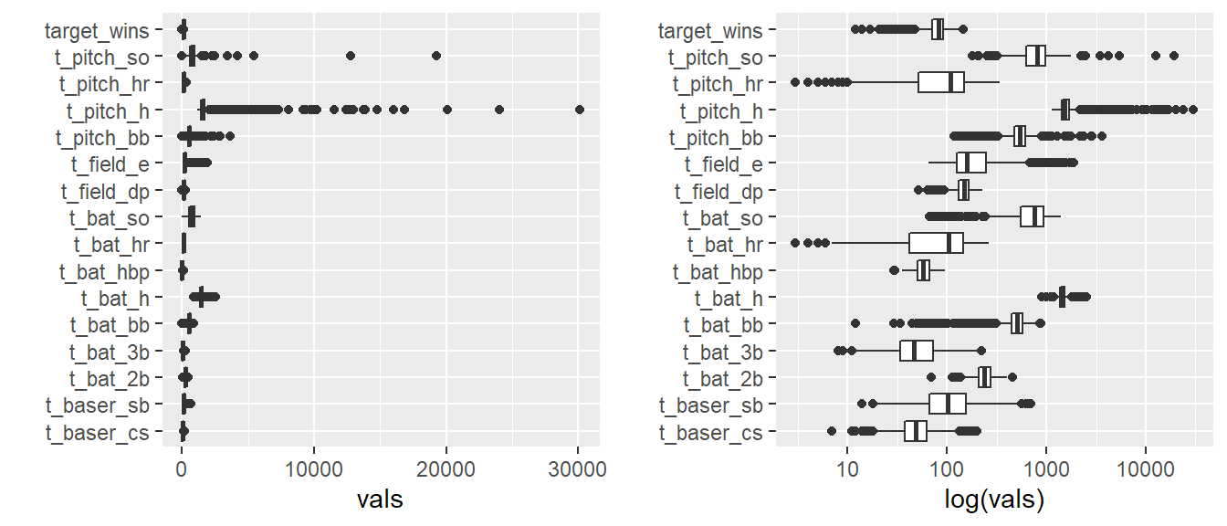
Note that the right-hand side plot is a duplicate of the left-hand plot but uses a log scale for the value-axis.
Multicollinearity
The below heat-map style plot highlights the correlation that exists between some of the predictor variables in the training set:
# check correlations between prediction vars:
# GGally::ggcorr(bsb_data[,c(6,8,12,13,15:17)],
#                geom = "circle", nbreaks = 6,
#                label=T, label_size = 3)
From the above plot above, selected variables and their respective correlation to other selected variables include:
TEAM_BATTING_HRandTEAM_BATTING_SO(HRs by batters and Strikeouts by batters)TEAM_BATTING_SOandTEAM_PITCHING_HR(Strikeouts by batters and HR’s allowed by pitchers)TEAM_BATTING_HRandTEAM_PITCHING_HR(HRs by batters and HRs allowed by pitch)TEAM_FIELDING_EandTEAM_PITCHING_H(Fielding errors and Hits allowed by pitchers)TEAM_FIELDING_DPandTEAM_FIELDING_E(Double-plays and fielding errors)
The presence of these values could indicate that some of these variables are doing ‘double-duty’ and may be removed in the fitting process with little loss of information.
Low Correlation To Response Variable
Pre-transformation TARGET_WINS vs. all other variables within the dataset in isoloation results in low correlation values and hints that transformations may be necessary in the modelling stage.
# see if there's cor btween target wins and others...
sm_tab <- cor(bsb_data[,-1]) %>% as.data.frame() %>%
  tibble::rownames_to_column(var = "var_name") %>%
  mutate(cor_val = round(target_wins , 4),
         abs_cor_val = abs(cor_val)) %>%
  select_("var_name", "abs_cor_val", "cor_val") %>%
  arrange(desc(abs_cor_val)) %>%
na.omit()| var_name | abs_cor_val | cor_val |
|---|---|---|
| target_wins | 1.0000 | 1.0000 |
| t_bat_h | 0.3888 | 0.3888 |
| t_bat_2b | 0.2891 | 0.2891 |
| t_bat_bb | 0.2326 | 0.2326 |
| t_pitch_hr | 0.1890 | 0.1890 |
| t_field_e | 0.1765 | -0.1765 |
Plotting all the variables against TARGET_WINS further highlights these low values:
bsb_data[,-1] %>%
  gather(-target_wins, key = "vars", value = "vals") %>%
  ggplot(aes(x = vals, y = target_wins)) +
    geom_point(alpha=.1) +
    facet_wrap(~ vars, scales = "free", ncol = 3)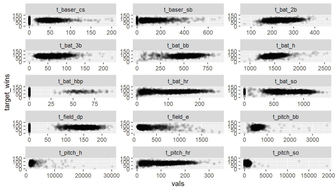
For convenience, the above plot was built by substituting 0’s for NA’s for all data but model fits do not. The primary takeaway is that in isolation, none of the variables appears to be a great predictor of TARGET_WINS.
Data Preperation
Several different methods were investigated. The below provides a summary of methods used to prepare each of the data-sets for 3 different model fits for the purpose of prediction.
na_ifelse <- function(x, metric){
  #function to replace NAs
  if(metric=="mean"){
    result = ifelse(is.na(x), mean(x, na.rm=T), x)
  }else if (metric == "med"){
    result = ifelse(is.na(x), median(x, na.rm=T), x)
  }else if (metric == "min"){
    result = ifelse(is.na(x), min(x, na.rm=T), x)
  }else
    result = ifelse(is.na(x), 0, x)
  return(result)
}
Below, I have outlined the steps taken to prepare individual data-sets for each model.
Model 1 Data:
Motivation: Based on the most complete set of records with minimal imputation:
- For
TEAM_BATTING_SOandTEAM_PITCHING_SO,NA-values replaced with themeanandmedianrespectively to address normal and skewed distributions respectively - these variables were only missing 4% of their records. - Removed
TEAM_BATTING_HBPbecause of its numerous missing values (92% of records missing values for this variable.)
f1_bsb_raw <- bsb_train_raw %>%
  mutate(t_bat_so = na_ifelse(t_bat_so, "mean"),
         t_pitch_so = na_ifelse(t_pitch_so, "med")) %>%
  select(-t_bat_hbp)
# sapply(new_bsb_raw, function(x) sum(is.na(x)))   # count na's per column!
# View(new_bsb_raw)
Model 2 Data:
Motivation: a refinement of the first model data-set that excludes variables that may be doing ‘double-duty’:
- Replace
NAwithmeanfor:TEAM_FIELD_DPto cover 13% of missing values - Replace
NAwithmedianforTEAM_PITCH_SOto cover 4% missing values - Remove
TEAM_BATTING_SObecause it’s highly correlated withTEAM_PITCHING_SO - Remove
TEAM_BASERUN_CSandTEAM_BATTING_HBPbecause 44% and 92% of records are missing respectively.
f2_bsb_raw <- bsb_train_raw %>%
  mutate(t_field_dp = na_ifelse(t_field_dp, "mean"),
         t_pitch_so = na_ifelse(t_pitch_so, "med")) %>%
  select(-t_bat_so, -t_baser_cs, -t_bat_hbp)
Model3 Data:
Motivation: Address all/most multicollinearity encountered and reduce the number of predictors overall to simplify the model. Variable selection between correlated predictors was based on ‘hitting-variables’ because those intuitively may result in more runs, and therefore, more wins.
- Remove
TEAM_BASERUN_CSandTEAM_BATTING_HBPbecause 44% and 92% of records are missing respectively. - Remove
TEAM_BATTING_2B/3B/HRasTEAM_BATTING_Hcovers all hit types - this is an attempt to simplify the model fit - Remove one side of the correlated pairs focusing on batting-related variables such that:
TEAM_BATTING_SOkept in, removedTEAM_PITCHING_SOTEAM_BATTING_Hkept in, removedTEAM_PITCHING_HTEAM_PITCHING_HRkept in, removedTEAM_BATTING_HRasTEAM_BATTING_Hcovers all hitsTEAM_FIELDING_Ekept in, removedTEAM_FIELDING_DP
f3_bsb_raw <- bsb_train_raw %>%
  select(-t_baser_cs, -t_bat_hbp,
         -t_bat_2b, -t_bat_3b, -t_bat_hr,
         -t_pitch_so, -t_pitch_h, -t_field_dp)


## A function to pull the coefficients from a linear model and present them nicely.
get_coefs <- function(an_lm){
  temp = an_lm$coefficients %>% as.data.frame()
  temp$Vars = rownames(temp)
  colnames(temp)[1] = "Coefs."
  rownames(temp) = NULL
  return(temp[,2:1])
}
Build Models
Model Fitting
Models were fit with the respective data-sets created in the previous section. Each section will display the resulting fit’s coefficients but the discussion of the coefficients will be saved for the Model Selection section.
Fit1:
Fit1 utilized the stepAIC function from the MASS package to perform step-wise model selection by AIC. I used this auto-selection method to investigate an off-the-shelf model’s performance with no additional transformations or imputation beyond what was originally discussed.
######## MODEL 1 FIT ########################
fitA <- lm(target_wins ~., f1_bsb_raw[,-1])
fitA_stepped <- MASS::stepAIC(fitA, trace=F)| Vars | Coefs. |
|---|---|
| (Intercept) | 58.4461 |
| t_bat_h | 0.0255 |
| t_bat_2b | -0.0698 |
| t_bat_3b | 0.1616 |
| t_bat_hr | 0.0977 |
| t_bat_bb | 0.0395 |
| t_baser_sb | 0.0360 |
| t_baser_cs | 0.0518 |
| t_pitch_h | 0.0091 |
| t_pitch_so | -0.0208 |
| t_field_e | -0.1560 |
| t_field_dp | -0.1131 |
#summary(fitA_stepped)
par(mfrow=c(1,2))
plot(fitA_stepped,which=c(2,1))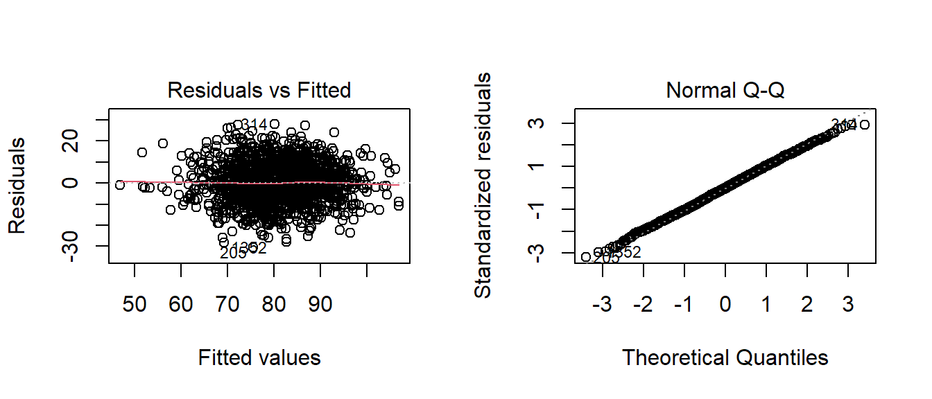
par(mfrow=c(1,1))Model 2 Fit:
An attempt at employing the powerTransform function from the car package to see if box-cox would yeild any transformation but my result was \(\lambda\approx1\) so I did not transform the model.
######## MODEL 2 FIT ########################
fitB <- lm(target_wins ~., f2_bsb_raw[,-1])
#fitB1 <- lm(target_wins+.01 ~., f2_bsb_raw[,-1])
#fitB_bc <- car::powerTransform(fitB1, family="bcPower") # 1.193639
#fitB_bc$roundlam # provides maximum estimator
#df <- cbind(lambda = fitB_bc$lambda, log_likli = fitB_bc$llik) %>% as.data.frame()
#df <- df %>% ungroup() %>% arrange(desc(log_likli))

#summary(fitB)| Vars | Coefs. |
|---|---|
| (Intercept) | 29.7307 |
| t_bat_h | 0.0422 |
| t_bat_2b | -0.0490 |
| t_bat_3b | 0.0741 |
| t_bat_hr | 0.0147 |
| t_bat_bb | 0.0303 |
| t_baser_sb | 0.0565 |
| t_pitch_h | 0.0027 |
| t_pitch_hr | 0.0557 |
| t_pitch_bb | -0.0030 |
| t_pitch_so | -0.0102 |
| t_field_e | -0.0517 |
| t_field_dp | -0.1168 |
par(mfrow=c(1,2))
plot(fitB,which=c(2,1))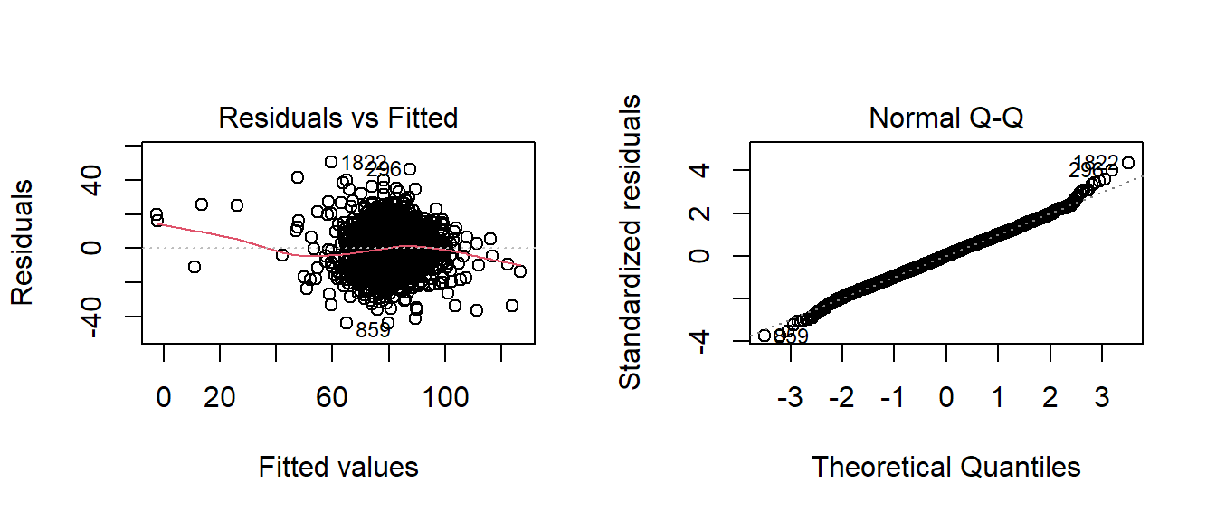
par(mfrow=c(1,1))Model 3 Fit:
The result of the box-cox transform here was a value of \(\lambda\approx1\) which again called for no transformation.
| Vars | Coefs. |
|---|---|
| (Intercept) | 24.3922 |
| t_bat_h | 0.0343 |
| t_bat_bb | 0.0239 |
| t_bat_so | -0.0160 |
| t_baser_sb | 0.0558 |
| t_pitch_hr | 0.0681 |
| t_pitch_bb | -0.0034 |
| t_field_e | -0.0346 |
Select Models
Criteria:
My selection criteria is based on comparing \(R^2\) and F-Statistics. If the performance is similar across these measures, I will select the model that is the easiest to describe of the two.
Model Selection:
I utilized the stargazer package to create the table below that compares Models 1, 2, and 3. Note that at the bottom of the table the models are compared by \(R^2\), adjusted \(R^2\), and the \(F\)-statistic.
stargazer(fitA_stepped,fitB, fitC,
          type='html',
          column.sep.width = "1pt",
          single.row = T,
          omit.stat=c('ser'),
no.space=TRUE)| Dependent variable: | |||
| target_wins | |||
| (1) | (2) | (3) | |
| t_bat_h | 0.026*** (0.006) | 0.042*** (0.004) | 0.034*** (0.003) |
| t_bat_2b | -0.070*** (0.009) | -0.049*** (0.009) | |
| t_bat_3b | 0.162*** (0.022) | 0.074*** (0.017) | |
| t_bat_hr | 0.098*** (0.009) | 0.015 (0.027) | |
| t_bat_bb | 0.039*** (0.003) | 0.030*** (0.006) | 0.024*** (0.004) |
| t_bat_so | -0.016*** (0.002) | ||
| t_baser_sb | 0.036*** (0.009) | 0.057*** (0.004) | 0.056*** (0.004) |
| t_baser_cs | 0.052*** (0.018) | ||
| t_pitch_h | 0.009*** (0.002) | 0.003*** (0.0004) | |
| t_pitch_hr | 0.056** (0.025) | 0.068*** (0.008) | |
| t_pitch_bb | -0.003 (0.004) | -0.003 (0.003) | |
| t_pitch_so | -0.021*** (0.002) | -0.010*** (0.002) | |
| t_field_e | -0.156*** (0.010) | -0.052*** (0.003) | -0.035*** (0.003) |
| t_field_dp | -0.113*** (0.013) | -0.117*** (0.012) | |
| Constant | 58.446*** (6.589) | 29.731*** (5.187) | 24.392*** (4.803) |
| Observations | 1,486 | 2,145 | 2,043 |
| R2 | 0.438 | 0.374 | 0.337 |
| Adjusted R2 | 0.434 | 0.370 | 0.335 |
| F Statistic | 104.596*** (df = 11; 1474) | 106.144*** (df = 12; 2132) | 147.644*** (df = 7; 2035) |
| Note: | p<0.1; p<0.05; p<0.01 | ||
Observations from these 3 models:
- None of the 3 models have very high \(R^2\) values.
- Each model’s F-statistic indicates that there is a relationship between predictor and the response variables included in the fits
Coefficients:
Model1: The intercept (‘Constant’) is too low for the mean value of TARGET_WINS but it’s not likely that every baseball team will get ~58 wins a season. The signs of the coefficients are problematic for several cases e.g. TEAM_BASERUN_CS (caught stealing) is positive but that would be detrimental to the wins and TEAM_FIELDING_E (fielding errors) are negative but fielding errors would lead to more on-bases and therefore, more runs.
Model2: More-intuitive intercept value but similarly un-intuitive coefficient signs that mirror the issues pointed out in Model1.
Model3: This model contains the fewest variables but 2 of them still have problematic signs including TEAM_FIELDING_E and TEAM_PITCHING_BB which I would expect to be positively correlated with wins.
Based on my criteria, since the performance of Model 1 is superior compared to the three models, I have selected Model 1.
Model Evaluation:
| Estimate | Std. Error | t value | Pr(>|t|) | |
|---|---|---|---|---|
| (Intercept) | 58.45 | 6.589 | 8.87 | 2.061e-18 |
| t_bat_h | 0.0255 | 0.005837 | 4.369 | 1.336e-05 |
| t_bat_2b | -0.06983 | 0.009292 | -7.515 | 9.857e-14 |
| t_bat_3b | 0.1616 | 0.02216 | 7.294 | 4.907e-13 |
| t_bat_hr | 0.09775 | 0.009435 | 10.36 | 2.516e-24 |
| t_bat_bb | 0.03948 | 0.003356 | 11.77 | 1.313e-30 |
| t_baser_sb | 0.03603 | 0.008668 | 4.157 | 3.407e-05 |
| t_baser_cs | 0.05177 | 0.0182 | 2.844 | 0.004511 |
| t_pitch_h | 0.00907 | 0.002353 | 3.855 | 0.0001205 |
| t_pitch_so | -0.02083 | 0.002312 | -9.006 | 6.419e-19 |
| t_field_e | -0.156 | 0.009917 | -15.73 | 1.205e-51 |
| t_field_dp | -0.1131 | 0.01312 | -8.623 | 1.653e-17 |
| Observations | Residual Std. Error | \(R^2\) | Adjusted \(R^2\) |
|---|---|---|---|
| 1486 | 9.548 | 0.4384 | 0.4342 |
The summary output from Model 1, above, reveals a number of challenges:
- The
Interceptvalue of ~ 60 could be too high given thatTARGET_WINScan take values as low as 0 (team loses all games) but it could also be too low given that themeanandmedianis \(approx\) 80. - The coefficients have very low p-values so the observed data is extremely unlikely to to have arisen if the the null hypothesis were true (i.e. that \(H_0: \beta_i = 0\) so we can reject the null hypothesis)
- 790 observations related to the missing values in columns
TEAM_BATTING_HBP - The \(R^2\) and multiple \(R^2\) values are low (\(R^2<.70\)) at \(\approx.43\) - this indicates to me that the data isn’t very close to the fitted regression and may provide poor predictions
- The negative coefficients under
TEAM_BATTING_2Band other base-gaining activities is counter-intuitive as getting on-base intuitively would result in more wins.
Below, the residual and QQ plots of Model1 appear to support a normal classification with some reservations. The residuals vs. the fitted plot appear to have a slight ‘kink’ when I expected an even, straight line. The normal QQ plot doesn’t deviate from the diagnol except in a few outlying cases.
par(mfrow=c(1,2))
plot(fitA_stepped,which=c(2,1))
par(mfrow=c(1,1))Model CI:
| 2.5 % | 97.5 % | |
|---|---|---|
| (Intercept) | 45.52 | 71.37 |
| t_bat_h | 0.01405 | 0.03695 |
| t_bat_2b | -0.08806 | -0.0516 |
| t_bat_3b | 0.1182 | 0.2051 |
| t_bat_hr | 0.07924 | 0.1163 |
| t_bat_bb | 0.0329 | 0.04607 |
| t_baser_sb | 0.01903 | 0.05304 |
| t_baser_cs | 0.01607 | 0.08747 |
| t_pitch_h | 0.004455 | 0.01368 |
| t_pitch_so | -0.02536 | -0.01629 |
| t_field_e | -0.1754 | -0.1365 |
| t_field_dp | -0.1389 | -0.08741 |
Prediction:
#READ IN EVALUATION DATA
bsb_eval_raw <- read_csv(mb_eval)
##
## -- Column specification --------------------------------------------------------
## cols(
## INDEX = col_double(),
## TEAM_BATTING_H = col_double(),
## TEAM_BATTING_2B = col_double(),
## TEAM_BATTING_3B = col_double(),
## TEAM_BATTING_HR = col_double(),
## TEAM_BATTING_BB = col_double(),
## TEAM_BATTING_SO = col_double(),
## TEAM_BASERUN_SB = col_double(),
## TEAM_BASERUN_CS = col_double(),
## TEAM_BATTING_HBP = col_double(),
## TEAM_PITCHING_H = col_double(),
## TEAM_PITCHING_HR = col_double(),
## TEAM_PITCHING_BB = col_double(),
## TEAM_PITCHING_SO = col_double(),
## TEAM_FIELDING_E = col_double(),
## TEAM_FIELDING_DP = col_double()
## )bsb_eval_raw <- data.table::setnames(bsb_eval_raw,
tolower(names(bsb_eval_raw[1:16])))
c1 <- col_name_updater(bsb_eval_raw, "batting", "bat")
c2 <- col_name_updater(c1, "pitching", "pitch")
c3 <- col_name_updater(c2, "fielding", "field")
c4 <- col_name_updater(c3, "baserun", "baser")
bsb_eval_raw <- col_name_updater(c4, "team", "t")
bsb_eval_raw <- bsb_eval_raw %>%
mutate(t_bat_so = na_ifelse(t_bat_so, "mean"),
t_pitch_so = na_ifelse(t_pitch_so, "med")) %>%
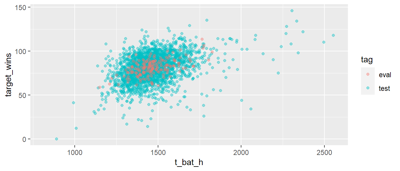
select(-t_bat_hbp)Below, I’ve used the evaluation data set, predicted the wins based on its ~200 records, and plotted the TARGET_WINS vs TEAM_BATTING_H. You can see the values wins predicted based on model 1 red in color.
# load test data into prediction
target_wins <- predict.lm(fitA_stepped, newdata=bsb_eval_raw[,-1])

# complete the test set
eval_set <- cbind(as.data.frame(target_wins),bsb_eval_raw[,-1]) %>%
  mutate(tag='eval')

tot_set <- f1_bsb_raw[,-1] %>%
  mutate(tag='test')

tot_set <- rbind(tot_set, eval_set)

x<-ggplot(tot_set, aes(x=t_bat_h, y=target_wins, color=tag)) +
  geom_point(alpha=.4)
x