LSTM for EMS Call Volume Prediction
Multivariate time-series forecasting is a non-trivial task when it comes to complex seasonality. Forecasting: Principles and Practice by R.J. Hyndman and G. Athanasopoulo, gives several powerful examples if you’re using R and dealing with seasonality using Fourier terms for each seasonal period (kinda like I did in this post).
In this post I’ll be using’s Keras RNN’s module for LSTM in python and forecasting the next 24 hours of call volume, per hour, into the future using the past 24 hours of my EMS data along with hourly weather data from Central Park via the NOAA. It’s going to be a basic model to present the basic steps.
Here’s a preview of the continuous variables:
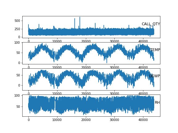
Feature Plot
And a preview of the cleaned data that made that plot:
In[1]: df.head()
Out[1]:
                     CALL_QTY  INC_DOW  INC_H  TEMP  DEWP         RH
INC_DAYH
2013-01-01 00:00:00     288.0      2.0    0.0  37.0  20.0  50.223652
2013-01-01 01:00:00     333.0      2.0    1.0  37.0  20.0  50.223652
2013-01-01 02:00:00     384.0      2.0    2.0  38.0  20.0  48.298279
2013-01-01 03:00:00     318.0      2.0    3.0  38.0  22.0  52.541706
2013-01-01 04:00:00     283.0      2.0    4.0  38.0  23.0  54.783157
Prepping the data:
import numpy as np
from numpy.random import seed
seed(123)
import pandas as pd
import matplotlib.pyplot as plt
from sklearn.preprocessing import MinMaxScaler
from sklearn.metrics import mean_absolute_error
from keras.models import Sequential
from keras.layers import LSTM, Dense
Preparing the time series data for Keras LSTM can be a bit of a challenge. If you face difficulty, I recommend this post post on Machine Learning Mastery - particularly his code for series_to_supervised function that allows for transposing your time series data.
Here it is reproduced from the above-mentioned post:
def series_to_supervised(data, n_in=1, n_out=1, dropnan=True):
    n_vars = 1 if type(data) is list else data.shape[1]
    df = pd.DataFrame(data)
    cols, names = list(), list()

    # input sequence (t-n, ... t-1)
    for i in range(n_in, 0, -1):
        cols.append(df.shift(i))
        names += [('var%d(t-%d)' % (j+1, i)) for j in range(n_vars)]
    # forecast sequence (t, t+1, ... t+n)
    for i in range(0, n_out):
        cols.append(df.shift(-i))
        if i == 0:
            names += [('var%d(t)' % (j+1)) for j in range(n_vars)]
        else:
            names += [('var%d(t+%d)' % (j+1, i)) for j in range(n_vars)]
    # put it all together
    agg = pd.concat(cols, axis=1)
    agg.columns = names
    # drop rows with NaN values
    if dropnan:
        agg.dropna(inplace=True)
    return agg
Once you understand how the algorithm structures the data, it is straight-forward for setting up the problem so that the neural network can interpret it.
forecastT = 24   # hours into the future
windowT   = 24   # hours into the past to use for prediction

# prep data for LSTM
allX = df.values
allY = df[['CALL_QTY']].values.reshape(-1,1)

# Use only the scaler fit on training portion for
# scaling the data.
# ~43817 hours
# ~1823 days
# 66% of 1823 days ~ 1203 days ~ 28872 hrs = training set
train_len = int(np.round(df.shape[0]*.66)) # 28919

## two different scalers
scalerX = MinMaxScaler(feature_range=(0, 1))
scalerY = MinMaxScaler(feature_range=(0, 1))

# use training set scaler on the test sets
scaledX = scalerX.fit_transform(allX[0:train_len, :])
scaledXte = scalerX.transform(allX[train_len:, :])

scaledY = scalerY.fit_transform(allY[0:train_len])
scaledYte = scalerY.transform(allY[train_len:])
Scaling the data improves the predictive performance of your model a great deal. Don’t forget to scale! Next I modify the results from series_to_supervised to fit the needs of my data. In particular, I need to clean up the column names before the merge operation to ensure I don’t overwrite my features.
valsx = np.concatenate((scaledX, scaledXte), axis = 0)
valsy = np.concatenate((scaledY, scaledYte), axis = 0)
rx = series_to_supervised(valsx, n_in = windowT)

# drop the actuals (hour 1) from the input features
rx = rx[rx.columns.drop(list(rx.filter(regex = "\(t\)")))]
ry = series_to_supervised(valsy, n_out = forecastT)

# drop the input feature CALL_QTY(t-1) that we already have in rx
ry.drop(columns = ["var1(t-1)"], inplace =True)
ry.columns = ry.columns.str.replace('var1', 'CQy')
# the input (x) is the past 24 hours of calls,
# temp, dewp, and RH.
# output (y) is the next 24 hours of calls only
rfull = pd.merge(rx, ry, left_index=True,
right_index=True, how="inner")
# After merging and dealing with the sliding window
# there are ~ 1,823 24 hour days included In[11]: rfull.head()
Out[11]:
var1(t-24) var2(t-24) var3(t-24) ... CQy(t+21) CQy(t+22) CQy(t+23)
24 0.438261 0.333333 0.000000 ... 0.234783 0.215652 0.168696
25 0.516522 0.333333 0.043478 ... 0.215652 0.168696 0.140870
26 0.605217 0.333333 0.086957 ... 0.168696 0.140870 0.085217
27 0.490435 0.333333 0.130435 ... 0.140870 0.085217 0.118261
28 0.429565 0.333333 0.173913 ... 0.085217 0.118261 0.076522
In[12]:rfull.shape
Out[12]: (43770, 168)Next I set up my get_naive forecast function that will extract var1 from the X data (i.e. the first column represents the past 24 hours of call quantities by hour):
## naive forecast repeats last 24 hours.
def get_naive(x):
    """
    Assumes x is type np.array of feature inputs only
    """
    result = []

    for i in range(0, np.shape(x)[1],
                   df.shape[1]):
        result.append(x[:, i].tolist())

    return(np.column_stack(result))
It will be used down the line for model diagnostics and performance measurements.
Training and Testing Split
Almost there: next I split the data up into testing and training sets:
# columns
fcols = len(rfull.columns)
ycols = len((rfull.filter(regex='CQ').columns))

# convert to np.array and split     \
values = rfull.values

train = values[:train_len, :]
test = values[train_len:, :]

# input/output split
train_X, train_y =  train[:, 0:(fcols - ycols)], train[:, (fcols - ycols):fcols]
test_X, test_y =  test[:, 0:(fcols - ycols)], test[:, (fcols - ycols):fcols]

# reshape input to be 3D [samples, timesteps, features] where:
# samples = number of rows (recall each row represents a 24hr slice)
# timesteps = how far back in the past we're using to forecast futre
# features = the original quantity of features in use.
train_X = train_X.reshape((train_X.shape[0], windowT, df.shape[1]))
test_X = test_X.reshape((test_X.shape[0], windowT, df.shape[1]))
Here are the batches created:
In[15]: print(train_X.shape, train_y.shape, test_X.shape, test_y.shape)
(28919, 24, 6) (28919, 24) (14851, 24, 6) (14851, 24)
LSTM Build
Now that the data is prepped and the testing/training data is ready I can build my model and evaluate it:
# Define model and fit it...
# Below is an LSTM with 50 neurons in the first hidden layer
# and 24 neurons in the output layer for predicting calls 24 hrs in adv.
# The input shape will be 24 time steps with 6 features.
# adam is the optimizer for learning rate
model = Sequential()
model.add(LSTM(50,
               input_shape=(train_X.shape[1], train_X.shape[2])))
model.add(Dense(forecastT))
#model.add(Dropout(.2))
model.compile(loss = "mae", optimizer = "adam")

# The model will be fit for 75 training epochs
# The internal state of the LSTM in Keras is reset
# at the end of each batch, so an internal state
# that is a function of a number of days - here, I choose 3
# days or 72 hours
history = model.fit(train_X, train_y, epochs=75,
                    batch_size= 72,
                    validation_data=(test_X, test_y),
                    verbose=2,
                    shuffle=False)
The above takes about 10 minutes on my Windows 7 machine to run. Here’s the plot of the history variable:
In[15]: plt.plot(history.history['loss'], label='train')
plt.plot(history.history['val_loss'], label='test')
plt.legend()
plt.show()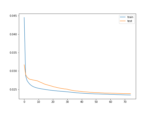
LSTM Train Test Eval
The plot seems to converge at approximately 0.025 mae (i.e. mean absolute error). This translates to roughly 4 calls per hour of the forecast.
Comparing with Actuals, Model Forecast, and Naive Forecast
Given the seasonal nature of the data (see this post for a look), I selected the input 24 hours of call quantities as the naive forecast (i.e. the naive forecast simply repeats same hours and call counts from the last 24 hours).
naivepreds = list()
for x in test_X:
    yhatn = get_naive(x).flatten()
    naivepreds.append(yhatn)

test_score_naive = mean_absolute_error(test_y, naivepreds)
test_score_model = mean_absolute_error(test_y, yhat)
And here are the results: MAE is a sensible choice given the non-Gaussian distribution of CALL_QTY in the data.
| MAE (Naive) | MAE (Model) |
|---|---|
| 0.039 | 0.024 |
While not a staggering improvement over the baseline, my model is more accurate than simply repeating the counts from the previous 24 hours. The naive forecast is about 6 calls in error while the model reduces that error to 3 calls per hour.
Here’s a random 24 hour period that compares the actuals, the forecast from the model, and the naive forecast on one plot:
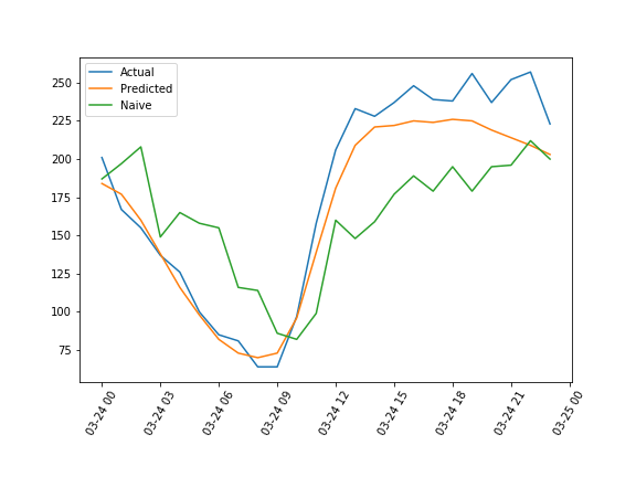
Actual v. Predicted v. Naive
Here’s the inverted transform of the 3 data sets described for the same time period:
                    Predicted  Actual  Naive
Date
2016-03-24 00:00:00      184.0   201.0  187.0
2016-03-24 01:00:00      177.0   167.0  197.0
2016-03-24 02:00:00      160.0   155.0  208.0
2016-03-24 03:00:00      138.0   137.0  149.0
2016-03-24 04:00:00      116.0   126.0  165.0
2016-03-24 05:00:00       98.0   100.0  158.0
2016-03-24 06:00:00       82.0    85.0  155.0
2016-03-24 07:00:00       73.0    81.0  116.0
2016-03-24 08:00:00       70.0    64.0  114.0
2016-03-24 09:00:00       73.0    64.0   86.0
2016-03-24 10:00:00       96.0    97.0   82.0
2016-03-24 11:00:00      139.0   158.0   99.0
2016-03-24 12:00:00      181.0   206.0  160.0
2016-03-24 13:00:00      209.0   233.0  148.0
2016-03-24 14:00:00      221.0   228.0  159.0
2016-03-24 15:00:00      222.0   237.0  177.0
2016-03-24 16:00:00      225.0   248.0  189.0
2016-03-24 17:00:00      224.0   239.0  179.0
2016-03-24 18:00:00      226.0   238.0  195.0
2016-03-24 19:00:00      225.0   256.0  179.0
2016-03-24 20:00:00      219.0   237.0  195.0
2016-03-24 21:00:00      214.0   252.0  196.0
2016-03-24 22:00:00      209.0   257.0  212.0
2016-03-24 23:00:00      203.0   223.0  200.0
Certainly this model can be improved but this post was mainly a demonstration on how Keras makes it very easy to apply neural networks to time series problems - highly recommended.