Linear Mixed Effect Models with lme4
This post is going to follow along and expand on a well-known tutorial for Mixed Effect Linear Models by Bodo Winters, a lecturer in Cognitive Linguistics at the University of Birmingham, Dept. of English Language and Applied Linguistics.
While this tutorial will generally follow Winter’s, I have added additional detail for EDA, expanded the details re: code & errors that are encountered, and added notes from many other sources on Mixed Effect Models (see the Sources section at the end for links) - let’s get started!
Pitch & Politeness Data
The tutorial on Mixed Effect Models by Bodo Winter makes use of an abbridged version of a data set that he collected in a Journal of Phonetics paper he authored titled: “The phonetic profile of Korean formal and informal speech registers” (Winter & Grawunder, 2012). The data was collected to study the relationship between pitch and politeness (you can find the original data for the paper here).
The primary library in this post is lme4. Among several ME packages in R, this one appears to be the most mature but it’s not a one-stop shop. You will need to become familiar with additional packages that support the merMod, a class of fitted mixed-effect models used by lme4 for diagnostics and more.
library(tidyverse)   # data wrangling
library(lme4)        # mixed effect models
library(merTools)    # Mixed effect model diagnostics
library(DHARMa)      # mixed effect model plots
library(lattice)     # mixed effect model plots
EDA
Overview
This data set is relatively small containing 84 observations:
pg <- read.csv("politedata.csv")
str(pg)
## 'data.frame': 84 obs. of 5 variables:
## $ subject : chr "F1" "F1" "F1" "F1" ...
## $ gender : chr "F" "F" "F" "F" ...
## $ scenario : int 1 1 2 2 3 3 4 4 5 5 ...
## $ attitude : chr "pol" "inf" "pol" "inf" ...
## $ frequency: num 213 204 285 260 204 ...The data includes 5 features:
subject: A code for a given participantgender: (M)ale or (F)emalescenario: Are numbers representing different scenarios recorded like when “asking for a favor” between a peer or a professorattitude: politeness levelfrequency: vocal pitch measured in Hertz where larger numbers mean higher-pitched
knitr::kable(pg %>% head(), format = 'html', booktabs = T)| subject | gender | scenario | attitude | frequency |
|---|---|---|---|---|
| F1 | F | 1 | pol | 213.3 |
| F1 | F | 1 | inf | 204.5 |
| F1 | F | 2 | pol | 285.1 |
| F1 | F | 2 | inf | 259.7 |
| F1 | F | 3 | pol | 203.9 |
| F1 | F | 3 | inf | 286.9 |
summary(pg)## subject gender scenario attitude
## Length:84 Length:84 Min. :1 Length:84
## Class :character Class :character 1st Qu.:2 Class :character
## Mode :character Mode :character Median :4 Mode :character
## Mean :4
## 3rd Qu.:6
## Max. :7
##
## frequency
## Min. : 82.2
## 1st Qu.:131.6
## Median :203.9
## Mean :193.6
## 3rd Qu.:248.6
## Max. :306.8
## NA's :1Further: this data set appears to be balanced and fully crossed - a characteristic that would be rare within real-world data.
xtabs(~ attitude + scenario, pg)## scenario
## attitude 1 2 3 4 5 6 7
## inf 6 6 6 6 6 6 6
## pol 6 6 6 6 6 6 6xtabs(~ attitude + gender, pg)## gender
## attitude F M
## inf 21 21
## pol 21 21xtabs(~ subject + gender, pg)## gender
## subject F M
## F1 14 0
## F2 14 0
## F3 14 0
## M3 0 14
## M4 0 14
## M7 0 14The continuous response variable here is frequency:
pg %>% ggplot(aes(x = frequency)) +
  geom_histogram(binwidth = 40, bins = 6,na.rm = T ) +
  labs(y = "Count", x = "Frequency (Hz)")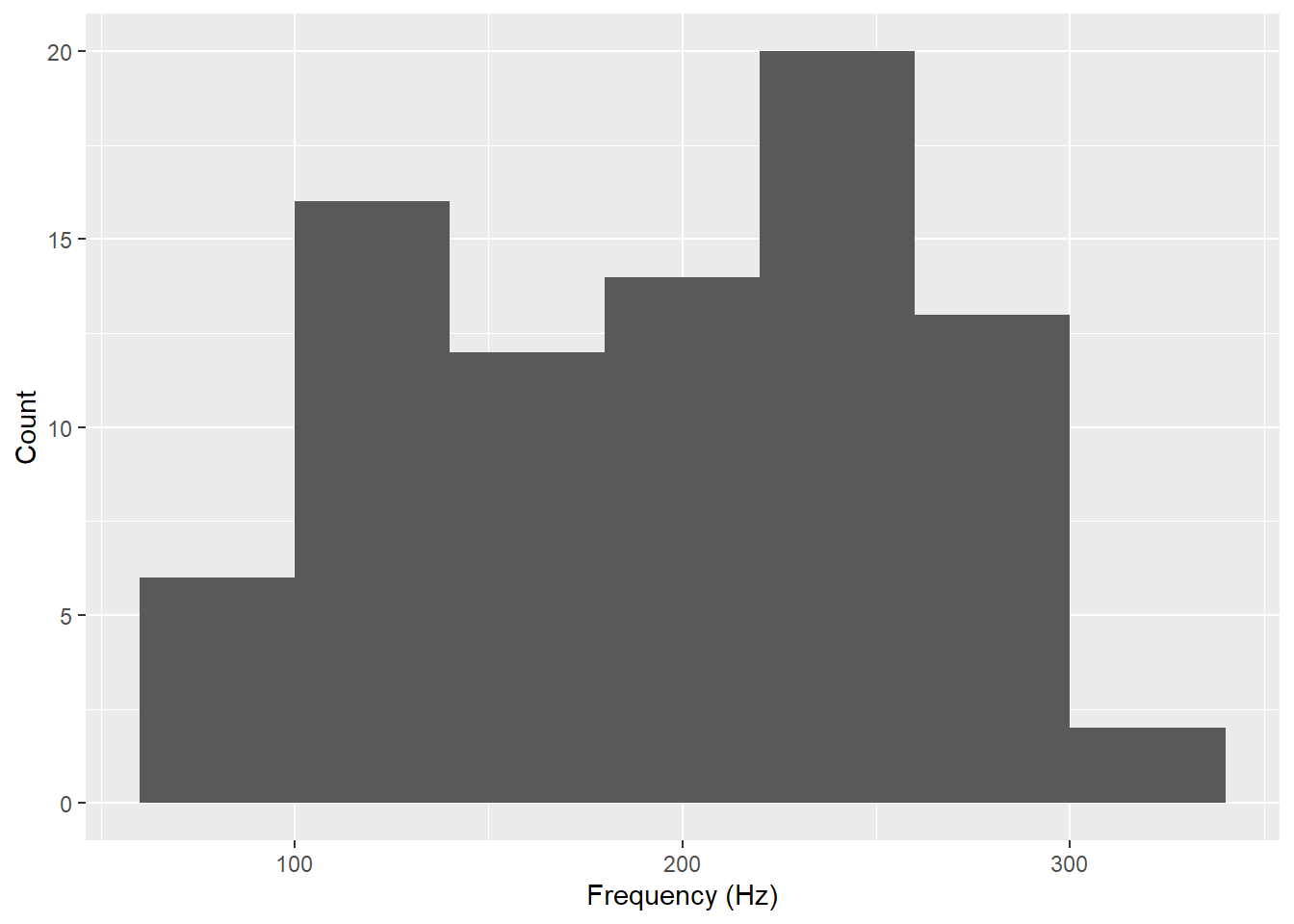
Missing Data
Only one missing value in this data seen here:
knitr::kable(pg[complete.cases(pg)==FALSE,], format = 'html')| subject | gender | scenario | attitude | frequency | |
|---|---|---|---|---|---|
| 39 | M4 | M | 6 | pol | NA |
I will simply drop the missing observation for the remainder of this post for simplification. If the sample size were larger, I would feel more comfortable in imputing this NA using the mean of the male subjects.
pg <- pg %>% drop_na()Gender
As expected, males have a lower vocal frequency than females:
pg %>% ggplot(aes(x = gender, y = frequency, fill = gender)) +
  geom_boxplot() +
  labs(y = "Frequency (Hz)", x = "Gender",
       fill = "Gender" )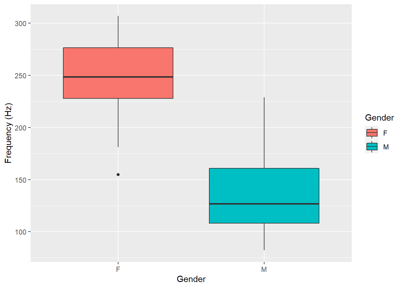
Furthermore, a plot of the interaction between gender and attitude for the scenarios also shows a relatively clear distinction for males and females:
pg %>%
  ggplot(aes(x = interaction(attitude, gender),
             y = frequency, fill = attitude)) +
  geom_boxplot(na.rm = T) +
  labs(y = "Frequency (Hz)", x = "Scenario & Gender Interaction",
       fill = "Attitude" )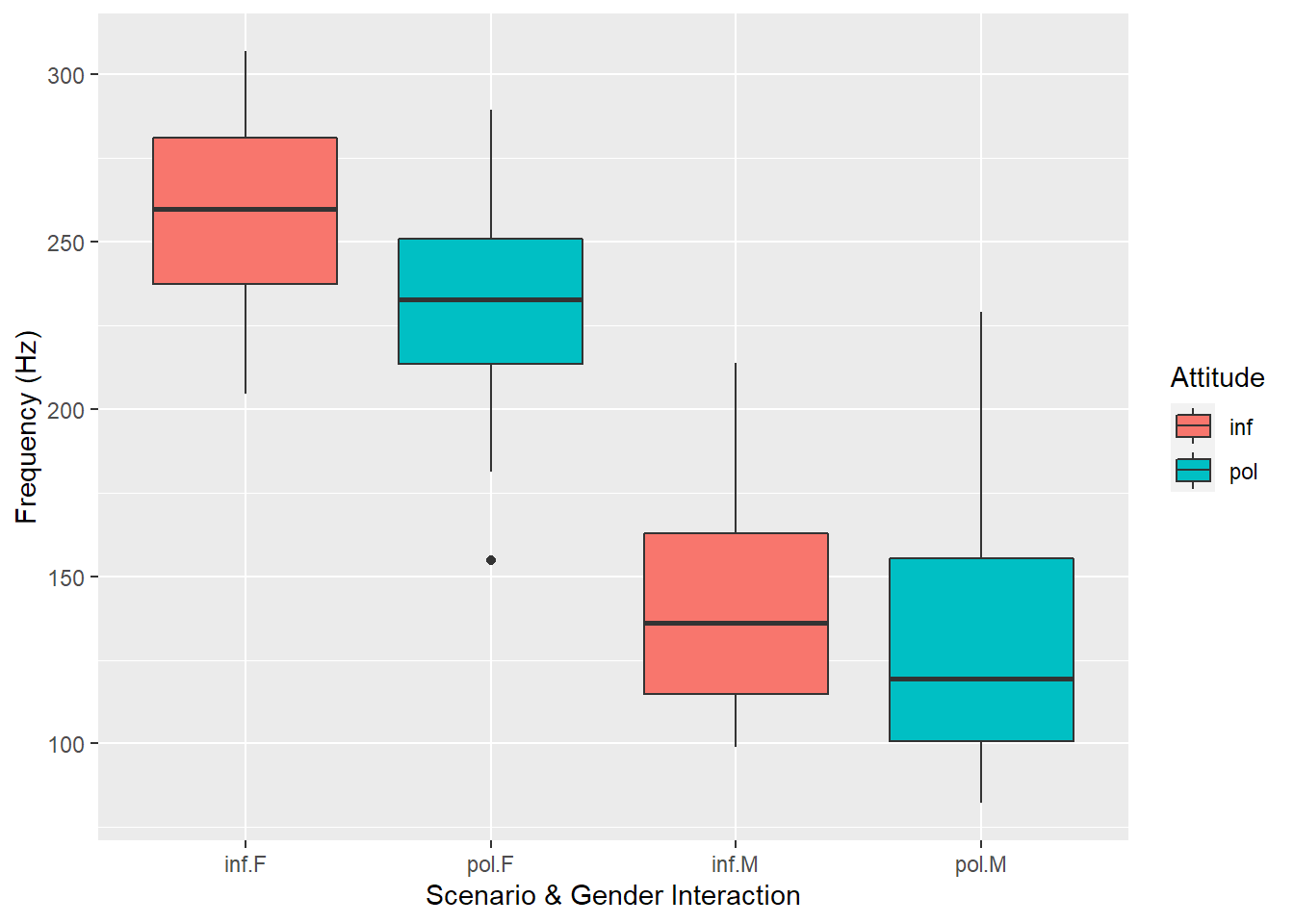
Subjects
And among these 6 subjects, the male/female vocal pitch differences are also clear:
pg %>%
  ggplot(aes(x = forcats::fct_reorder(subject,
                                      frequency,
                                      median),
                  y =frequency, fill = gender)) +
  geom_boxplot(na.rm = T) +
  labs(y = "Frequency (Hz)", x = "Subject",
       fill = "Gender" )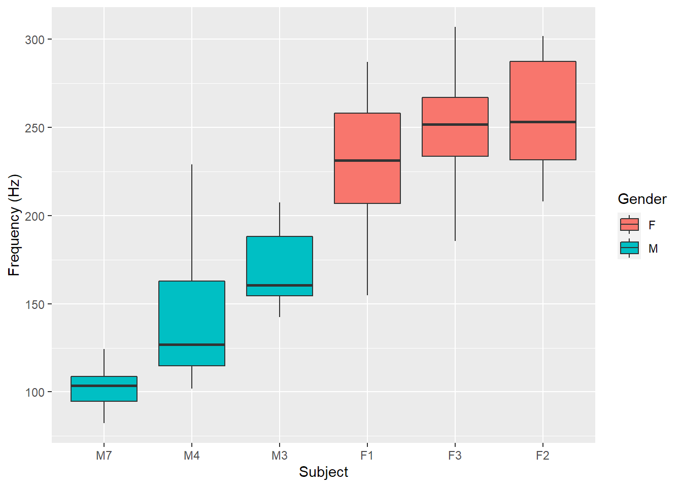
Attitude
When reviewing the vocal frequencies of all observations between attitudes (where inf= informal and pol = polite), we can see that overall, informal attitudes have a higher pitch than the formal ones:
pg %>% ggplot(aes(x = attitude, y = frequency,
                  fill = attitude)) +
  geom_boxplot(na.rm = T) +
  labs(y = "Frequency (Hz)", x = "Attitude",
       fill = "Attitude" )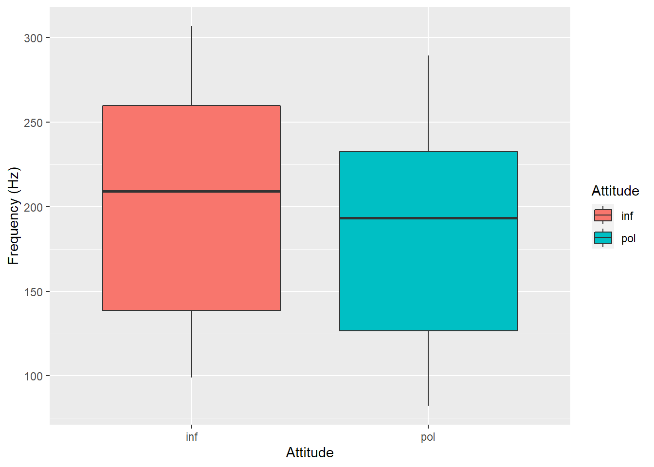
For almost all of the subjects except for M2, the frequency drops between attitudes informal (inf) to polite (pol):
pg %>%
  ggplot(aes(x=attitude, y=frequency)) +
  facet_wrap(~subject,
             ncol=3, scales='free')  +
  geom_point()+
  stat_smooth(method='lm', aes(group=1)) +
  labs(y = "Frequency (Hz)", x = "Attitude",
       title = "Frequency vs Attitude by Subject")
## `geom_smooth()` using formula 'y ~ x'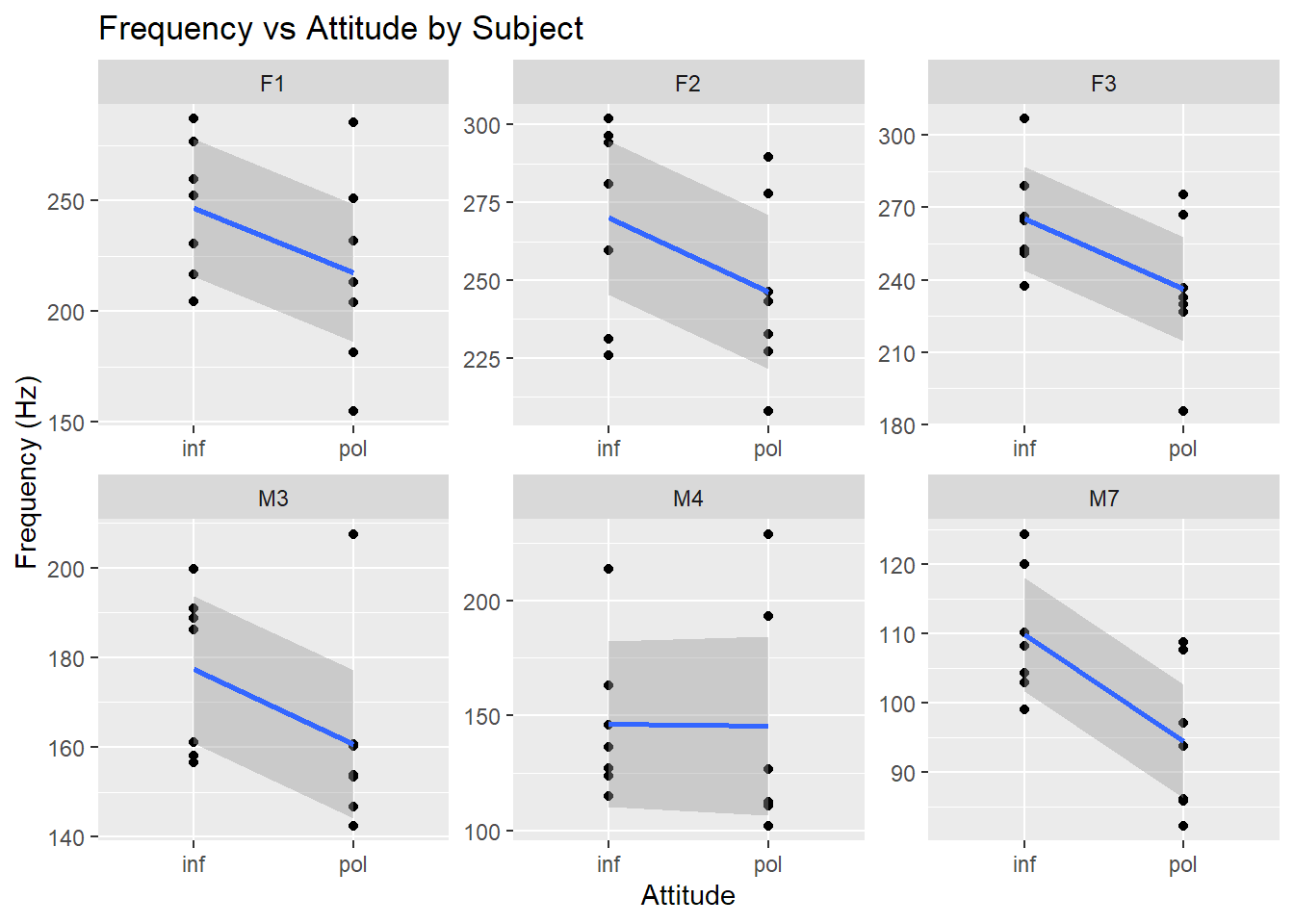
Scenarios
Scenarios in isolation appear to result in differing vocal pitch ranges:
pg %>%
  ggplot(aes(x = as.factor(scenario),
             y = frequency, fill = as.factor(scenario))) +
  geom_boxplot(na.rm = T) +
  labs(y = "Frequency (Hz)", x = "Scenario",
       fill = "Scenario")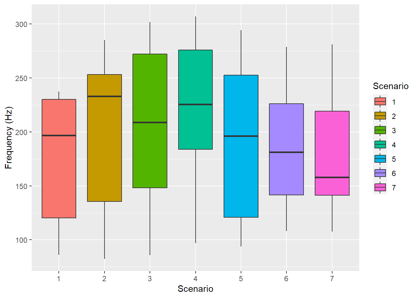
We can see that the frequency differs among the scenarios grouped by attitude in the observations as well:
pg %>%
  ggplot(aes(x = as.factor(scenario),
             y = frequency, fill = attitude)) +
  geom_boxplot(na.rm = T) +
  labs(y = "Frequency (Hz)", x = "Scenario",
       fill = "Attitude" )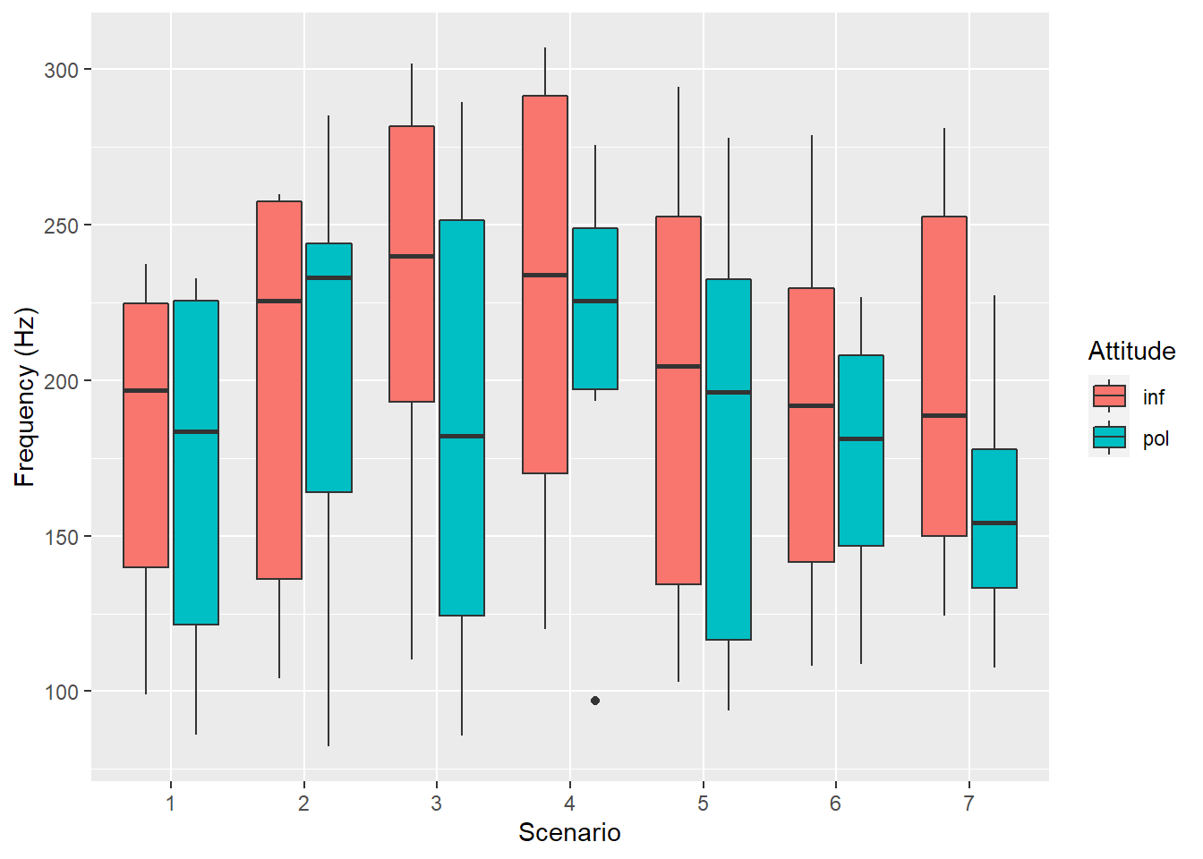
Among the scenarios, frequency generally drops between informal (inf) and polite (pol) except for scenario 2:
pg %>%
  ggplot(aes(x=attitude, y=frequency)) +
  facet_wrap(~scenario, #interaction(gender, scenario),
             ncol=4, scales='free') +
  geom_point()+
  stat_smooth(method='lm', aes(group=1)) +
  labs(y = "Frequency (Hz)", x = "Attitude",
       title = "Frequency vs Attitude by Scenario")
## `geom_smooth()` using formula 'y ~ x'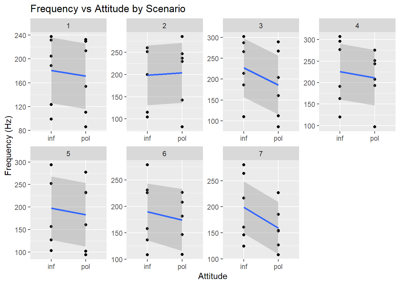
Random Intercept Models
In short, Mixed Models are regression models that contain both random and fixed effects. In mixed models, fixed effects are treated similarly to how observations are treated in linear regression i.e. the independence assumptions for observations must hold. However, when faced with scenarios that include multiple observations from the same person (e.g. one student’s test scores among several tests), we end up breaking the independence assumptions for linear regression. This is where random affects come in.
If we had a classroom of students and we were looking to model test scores among the class using individuals student scores across several tests, the test scores associated with specific students are not independent.
To deal with this inter-dependency between observations (the same student across different tests) we can used the Random Effects within a mixed model. These random effects allow us to create student-specific random variables (e.g. intercepts, or mean test scores per student) that are applied depending on the student. The student-specific random effects in a mixed model allows us to maintain the independence requirement for linear regression.
Model 1
EDA revealed that there are a number of variables that are good candidates to model as random effects. These are features that are not independent of each other among multiple readings like subject and scenario (i.e. multiple readings from the same subject are not independent and multiple readings from the same scenario are also not independent).
m1 <- lmer(frequency ~ attitude +
             (1|subject) + (1|scenario), data = pg)
Next we review the summary of m1:
# summary(m1)
fastdisp(m1)
## lmer(formula = frequency ~ attitude + (1 | subject) + (1 | scenario),
## data = pg)
## coef.est coef.se
## (Intercept) 202.59 26.75
## attitudepol -19.69 5.58
##
## Error terms:
## Groups Name Std.Dev.
## scenario (Intercept) 14.80
## subject (Intercept) 63.36
## Residual 25.42
## ---
## number of obs: 83, groups: scenario, 7; subject, 6
## AIC = 803.5Fixed Effect m1
The first part of the output from fastdisp(m1) displays the fixed effect terms including the (Intercept)- the average frequency from the data grouped by attitude:
knitr::kable(pg %>%
  group_by(attitude) %>%
  summarise(`Mean Frequency` = mean(frequency)),
format = 'html')| attitude | Mean Frequency |
|---|---|
| inf | 202.5881 |
| pol | 184.3561 |
The next part include the attitudepol - the slope of the model dependent on the attitude. The negative slope indicated by attitudepol shows that in moving from inf to pol, the vocal pitch drops by ~20Hz (based on the alphabetical order of the levels within the attitude factor). Using the general summary() function would have additionally revealed the t-value for attitudepol calculated by dividing the slope by the coef.se (-19.695/5.585 = -3.52641).
Random Effects m1
The standard deviation of the Error terms above are related to the random effects defined in m1. The non-zero values for scenario and subject reveal that there is variability in frequency related to both of these effects (values very close to zero would indicate that the random effect variables weren’t changing the prediction and that are selection for random effects wasn’t great).
In particular, scenario appears to have less of an impact on frequency than test subject (14.80 < 63.36). Furthermore, the Residual standard deviation reveals that there is variation in frequency that’s not accounted for by either random effect scenario or subject.
Model 2
For the next model, we add gender to fixed effects. Like attitude the category of gender has clear, systemic distinctions (i.e. men’s vocal pitch is lower than females vocal pitch as seen during EDA under “Gender”).
m2 <- lmer(frequency ~ attitude + gender +
           (1|subject) + (1|scenario),
           data = pg)
# summary(m2)
fastdisp(m2)## lmer(formula = frequency ~ attitude + gender + (1 | subject) +
## (1 | scenario), data = pg)
## coef.est coef.se
## (Intercept) 256.85 16.12
## attitudepol -19.72 5.58
## genderM -108.52 21.01
##
## Error terms:
## Groups Name Std.Dev.
## scenario (Intercept) 14.81
## subject (Intercept) 24.81
## Residual 25.41
## ---
## number of obs: 83, groups: scenario, 7; subject, 6
## AIC = 787.5Fixed Effect m2
While the slope associated with attitudepol hasn’t changed much from m1, the slope indicated by genderM shows that moving from F to M indicates a frequency drop of ~108.5 Hz - exactly as expected from EDA.
Random Effects m2
After adding the fixed effect from gender, the standard deviation for random effect subject has dropped from 63.36 (m1) to 24.81 (m2).
So is m2 a better model than m1? We can use an anova() to help us confirm. Keep in mind that the one should confirm assumptions of linearity:
m1 <- lmer(frequency ~ attitude +
             (1|subject) + (1|scenario),
           data = pg, REML = F)
m2 <- lmer(frequency ~ attitude + gender +
             (1|subject) + (1|scenario),
           data = pg, REML = F)
anova(m1,m2)
## Data: pg
## Models:
## m1: frequency ~ attitude + (1 | subject) + (1 | scenario)
## m2: frequency ~ attitude + gender + (1 | subject) + (1 | scenario)
## npar AIC BIC logLik deviance Chisq Df Pr(>Chisq)
## m1 5 817.04 829.13 -403.52 807.04
## m2 6 807.10 821.61 -397.55 795.10 11.938 1 0.00055 ***
## ---
## Signif. codes: 0 '***' 0.001 '**' 0.01 '*' 0.05 '.' 0.1 ' ' 1# Note that fitting model(s) with REML = F
# allows for the anova test to function.
# It does alter the summary output info in default. Hypothesis Testing:
The first model (Null Model) is fitted without the variable of interest and the second model is fitted with the variable of interest. You can then use the Likelihood Ratio Test as a means to attain p-values and see if the variable of interest is statistically significant.
Recall that Likelihood is the probability of seeing the data that was collected given the model under investigation. The likelihood ratio test compares the likelihood of two models with each other.
Testing significance of attitude with Random Intercept Model:
Next we look to test the significance of attitude in impacting the vocal frequency. I’ll fit a model without attitude (null) and then fit a model with attitude and then compare them using the Likelihood Ratio Test via anova():
# Include REML=FALSE when fitting for Liklihood Ratio Tests
m1.null <- lmer(frequency ~ gender + (1|subject) + (1|scenario),
               data=pg, REML=FALSE)#, verbose = 10)
m1.altr <- lmer(frequency ~ attitude + gender +
                  (1|subject) + (1|scenario),
                data=pg, REML=FALSE)
Next we complete the test :
# Always put less-complex model first in the anova() function:
anova(m1.null,m1.altr)
## Data: pg
## Models:
## m1.null: frequency ~ gender + (1 | subject) + (1 | scenario)
## m1.altr: frequency ~ attitude + gender + (1 | subject) + (1 | scenario)
## npar AIC BIC logLik deviance Chisq Df Pr(>Chisq)
## m1.null 5 816.72 828.81 -403.36 806.72
## m1.altr 6 807.10 821.61 -397.55 795.10 11.618 1 0.0006532 ***
## ---
## Signif. codes: 0 '***' 0.001 '**' 0.01 '*' 0.05 '.' 0.1 ' ' 1For convenience, I’m reprinting the summary from m1.altr as it’s referenced in the next section:
fastdisp(m1.altr)## lmer(formula = frequency ~ attitude + gender + (1 | subject) +
## (1 | scenario), data = pg, REML = FALSE)
## coef.est coef.se
## (Intercept) 256.85 13.83
## attitudepol -19.72 5.55
## genderM -108.52 17.57
##
## Error terms:
## Groups Name Std.Dev.
## scenario (Intercept) 14.33
## subject (Intercept) 20.42
## Residual 25.25
## ---
## number of obs: 83, groups: scenario, 7; subject, 6
## AIC = 807.1Using the summary of the anova Chi-Square value, the associated degrees of freedom (Df = the number of features in the alternative hypothesis - in this case 1), and the associated summary of m1.altr, the results of the test can be stated as follows:
`attitude` affected pitch (chi^2(Df=1) = 11.618, p = .0006532) by about -19.72 Hz +/- 5.6 standard errors.Random Slope Model
Reviewing the coefficients of the m1.altr, we see that we created a model that allows for different baseline frequency values for scenario and subject but that the slopes for attitudepol and genderM are fixed.
coef(m1.altr)## $scenario
## (Intercept) attitudepol genderM
## 1 243.4860 -19.72207 -108.5173
## 2 263.3592 -19.72207 -108.5173
## 3 268.1322 -19.72207 -108.5173
## 4 277.2546 -19.72207 -108.5173
## 5 254.9319 -19.72207 -108.5173
## 6 244.8015 -19.72207 -108.5173
## 7 245.9618 -19.72207 -108.5173
##
## $subject
## (Intercept) attitudepol genderM
## F1 243.3684 -19.72207 -108.5173
## F2 266.9442 -19.72207 -108.5173
## F3 260.2276 -19.72207 -108.5173
## M3 284.3535 -19.72207 -108.5173
## M4 262.0575 -19.72207 -108.5173
## M7 224.1293 -19.72207 -108.5173
##
## attr(,"class")
## [1] "coef.mer"However, in the real world such static relationships of this type are unlikely. For example, test subjects may have different rates of changes in vocal frequency between pol and inf or between their gender M and F - recall the plot from EDA.
Furthermore, each scenario may elicit different rates of change in frequency depending on attitude and gender as well.
What this means is that to get a better grasp that attitude is significant in determining vocal pitch, we need to investigate its significance with a model that allows for these changes.
Testing significance of attitude with Random Slope Model:
Addressing the fixed effects in random intercept models accounted only for the baseline deltas between for gender and attitude. By also allowing for random slopes dependent on the subject and scenario, we can further confirm the significance of attitude:
# if your full model is a random slope model,
# your null model also needs to be a random
# slope model

m3.null = lmer(frequency ~ gender +
                 (1+attitude|subject) + (1+attitude|scenario),
               data =pg, REML=FALSE)
## boundary (singular) fit: see ?isSingular# NOTE:
# The failure to converge for m3.null is a false positive via:
# m3.null.all <- allFit(m3.null)
# ss <- summary(m3.null.all)
# ss$ fixef ## fixed effects >> All roughly the same
# ss$ llik ## log-likelihoods >> All roughly the same
# ss$ sdcor ## SDs and correlations >> All roughly the same
# ss$ theta ## Cholesky factors >> All roughly the same
# ss$ which.OK ## which fits worked >> All but 1: optimx.L-BFGS-B
# Below the (1+a|b) notation means that each subject gets
# its own intercept
m3.altr <- lmer(frequency ~ attitude + gender +
(1+attitude|subject) + (1+attitude|scenario),
data=pg, REML=FALSE)## boundary (singular) fit: see ?isSingularanova(m3.null, m3.altr)## Data: pg
## Models:
## m3.null: frequency ~ gender + (1 + attitude | subject) + (1 + attitude |
## m3.null: scenario)
## m3.altr: frequency ~ attitude + gender + (1 + attitude | subject) + (1 +
## m3.altr: attitude | scenario)
## npar AIC BIC logLik deviance Chisq Df Pr(>Chisq)
## m3.null 9 819.61 841.37 -400.80 801.61
## m3.altr 10 814.90 839.09 -397.45 794.90 6.7082 1 0.009597 **
## ---
## Signif. codes: 0 '***' 0.001 '**' 0.01 '*' 0.05 '.' 0.1 ' ' 1Again Likelihood Ratio Test has confirmed that attitude is significant in impacting vocal pitch in the model. In addition, the AIC of m3.altr indicates that this model fits the data better than the null model. I’ll print out the summary of m3.altr so that I can report the results.
# Here I use the full summary as it provides
# additonal information
summary(m3.altr)
## Linear mixed model fit by maximum likelihood ['lmerMod']
## Formula: frequency ~ attitude + gender + (1 + attitude | subject) + (1 +
## attitude | scenario)
## Data: pg
##
## AIC BIC logLik deviance df.resid
## 814.9 839.1 -397.4 794.9 73
##
## Scaled residuals:
## Min 1Q Median 3Q Max
## -2.1946 -0.6690 -0.0789 0.5256 3.4251
##
## Random effects:
## Groups Name Variance Std.Dev. Corr
## scenario (Intercept) 182.083 13.494
## attitudepol 31.244 5.590 0.22
## subject (Intercept) 392.344 19.808
## attitudepol 1.714 1.309 1.00
## Residual 627.890 25.058
## Number of obs: 83, groups: scenario, 7; subject, 6
##
## Fixed effects:
## Estimate Std. Error t value
## (Intercept) 257.991 13.528 19.071
## attitudepol -19.747 5.922 -3.335
## genderM -110.806 17.510 -6.328
##
## Correlation of Fixed Effects:
## (Intr) atttdp
## attitudepol -0.105
## genderM -0.647 0.003
## optimizer (nloptwrap) convergence code: 0 (OK)
## boundary (singular) fit: see ?isSingularThe findings from this test would be reported as:
`attitude` affected pitch (chi^2(Df=1) = 6.7082, p = 0.009597) by about -19.75 Hz +/- 5.9 standard errors.Diagnostics
Model diagnostics are generally performed throughout the process of model building/development but I’m putting them at the end here for reference. There are number of ways to test that a given mixed model properly conforms to the requirements for linearity. Here are a few for the m3.altr model we created:
Independence
Mixed models are used to avoid or resolve the violation of the independence assumption that arises from repeated observations of the same subject. However, using mixed models doesn’t mean that you’re automatically in the clear because you can still violate the independence assumption with mixed models. If the m3.altr didn’t include a random effect for subject our model isn’t accounting for repeated measure and that’s a violation of the independence assumption right there. All inferences/conclusions made from this model are going to be over-confident. Careful consideration of the data under investigation must be made to ensure that you’re not violating the independence assumption.
###Linearity
Here’s the fitted vs the residuals
pdata <- data.frame(pg %>%
                      drop_na(),
                    fitted=fitted(m3.altr),
                    resid=residuals(m3.altr))
xyplot(fitted~resid,data=pdata)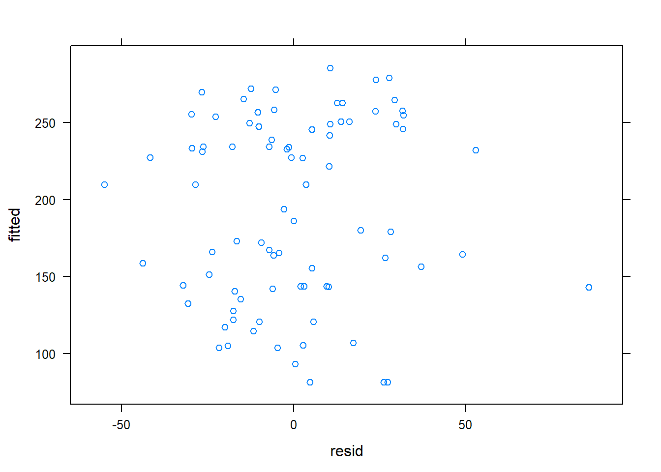
This residual plot does not indicate any patterns so we can say this assumption is met.
Recall that we still need to maintain linearity but because this is a mixed model, we need to ensure independence by groups and that they’re uncorrelated:
Homogeneity of Variance
Below, the residuals appear evenly and randomly sprinkled about the zero line.
plot(m3.altr)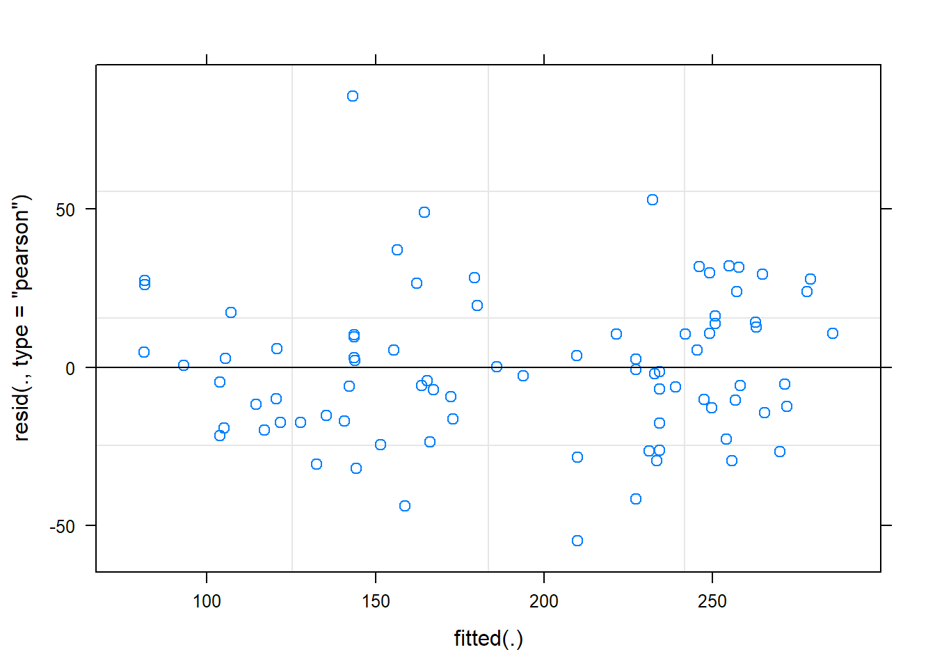
We can check for homogeneity among the different categories as well:
plot(m3.altr,
     resid(., scaled=TRUE) ~ fitted(.) | attitude, abline = 0)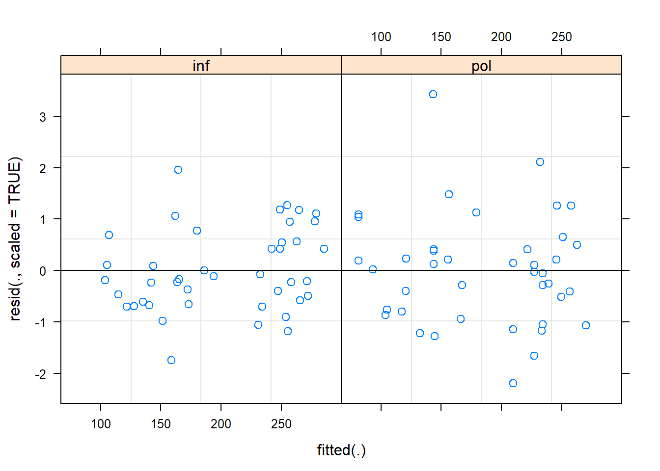
plot(m3.altr,
     resid(., scaled=TRUE) ~ fitted(.) | subject, abline = 0)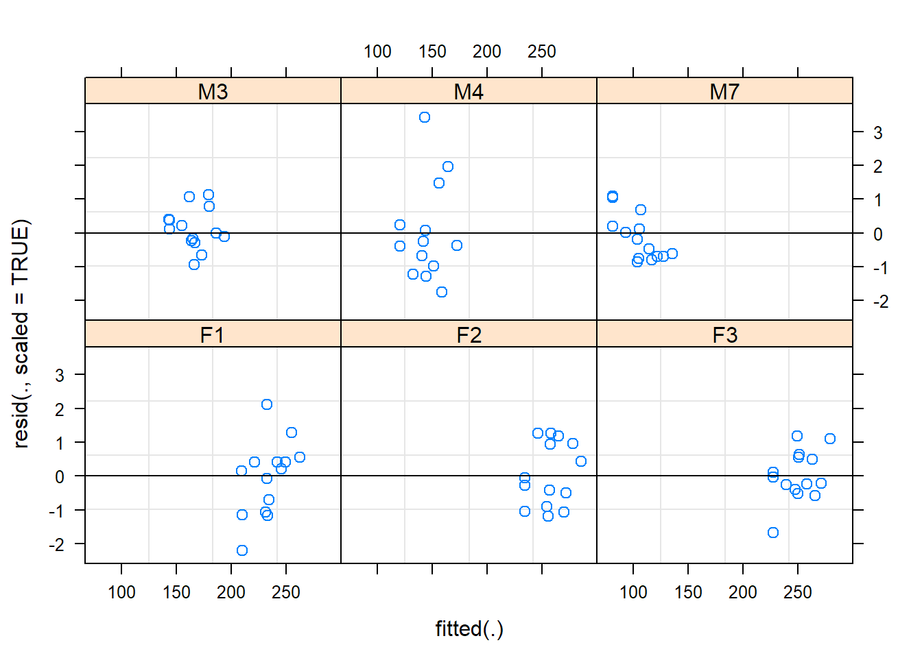
plot(m3.altr,
     resid(., scaled=TRUE) ~ fitted(.) | scenario, abline = 0)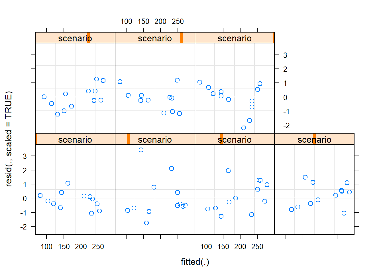
plot(m3.altr,
     resid(., scaled=TRUE) ~ fitted(.) | gender, abline = 0)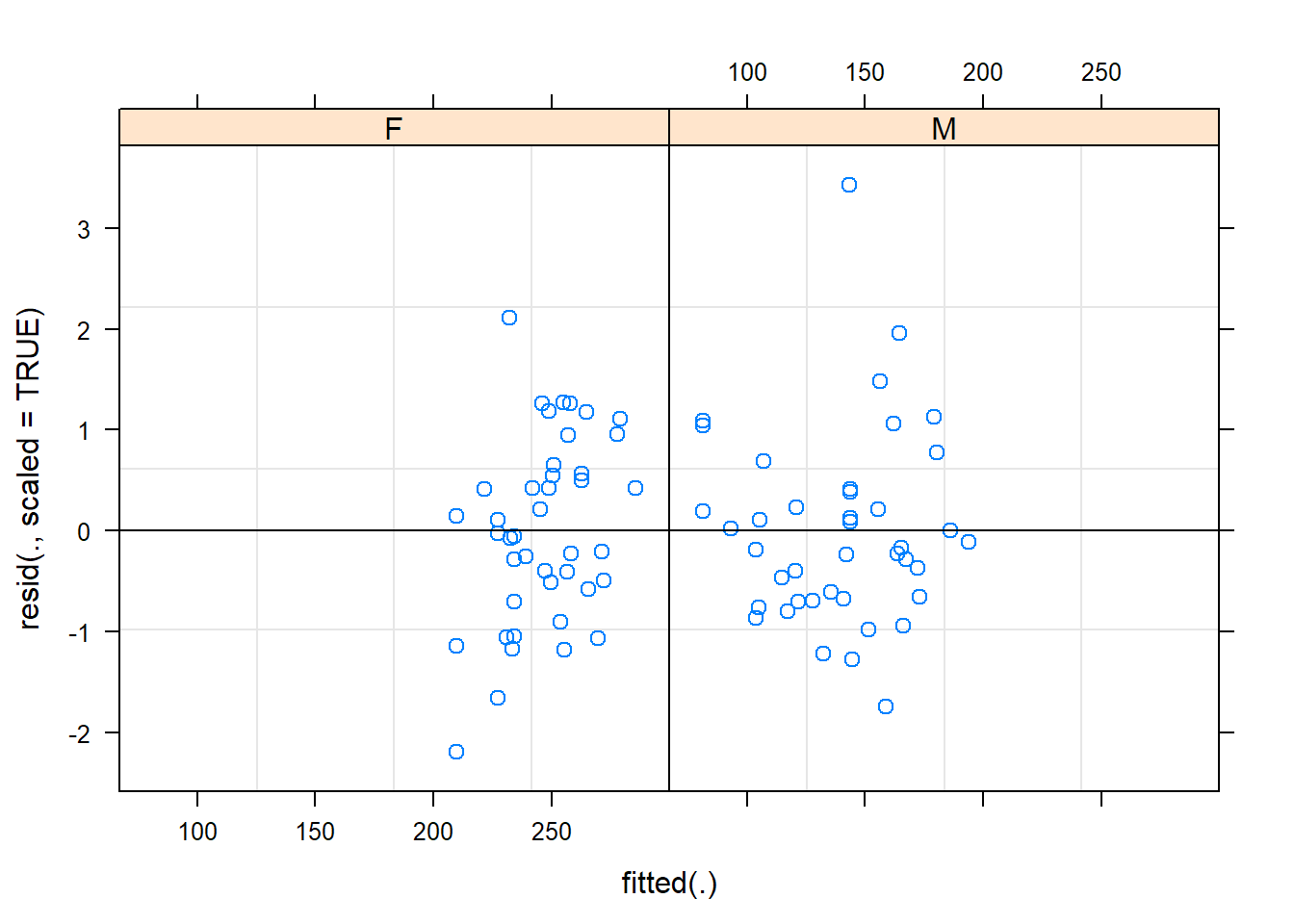
Normality of Residuals
The Normal QQ plot doesn’t show wild swings from normality except for the tails and this is a satisfactory result.
hist(residuals(m3.altr))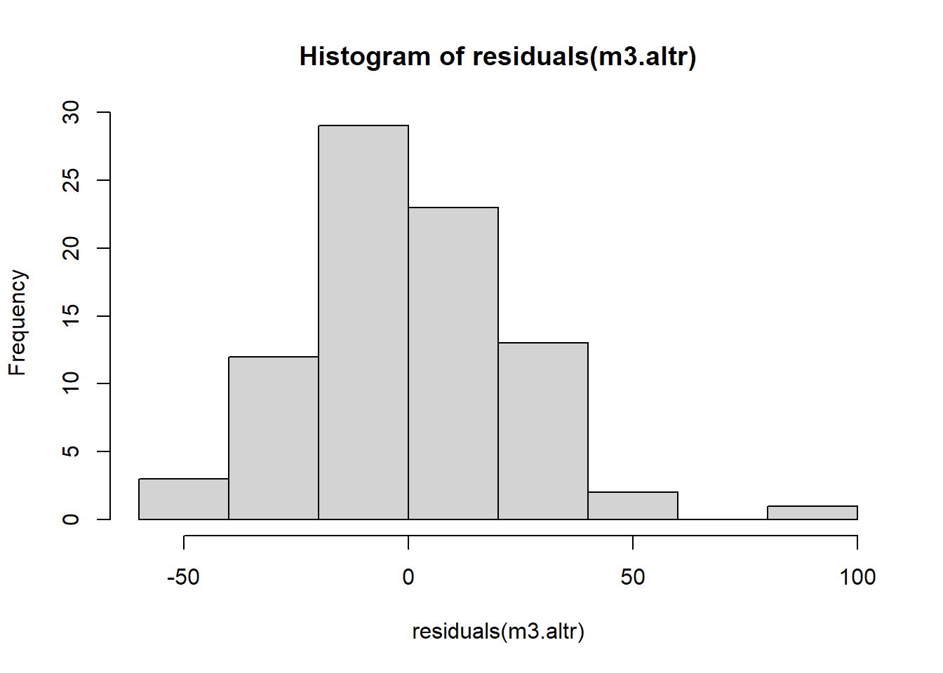
qqnorm(residuals(m3.altr))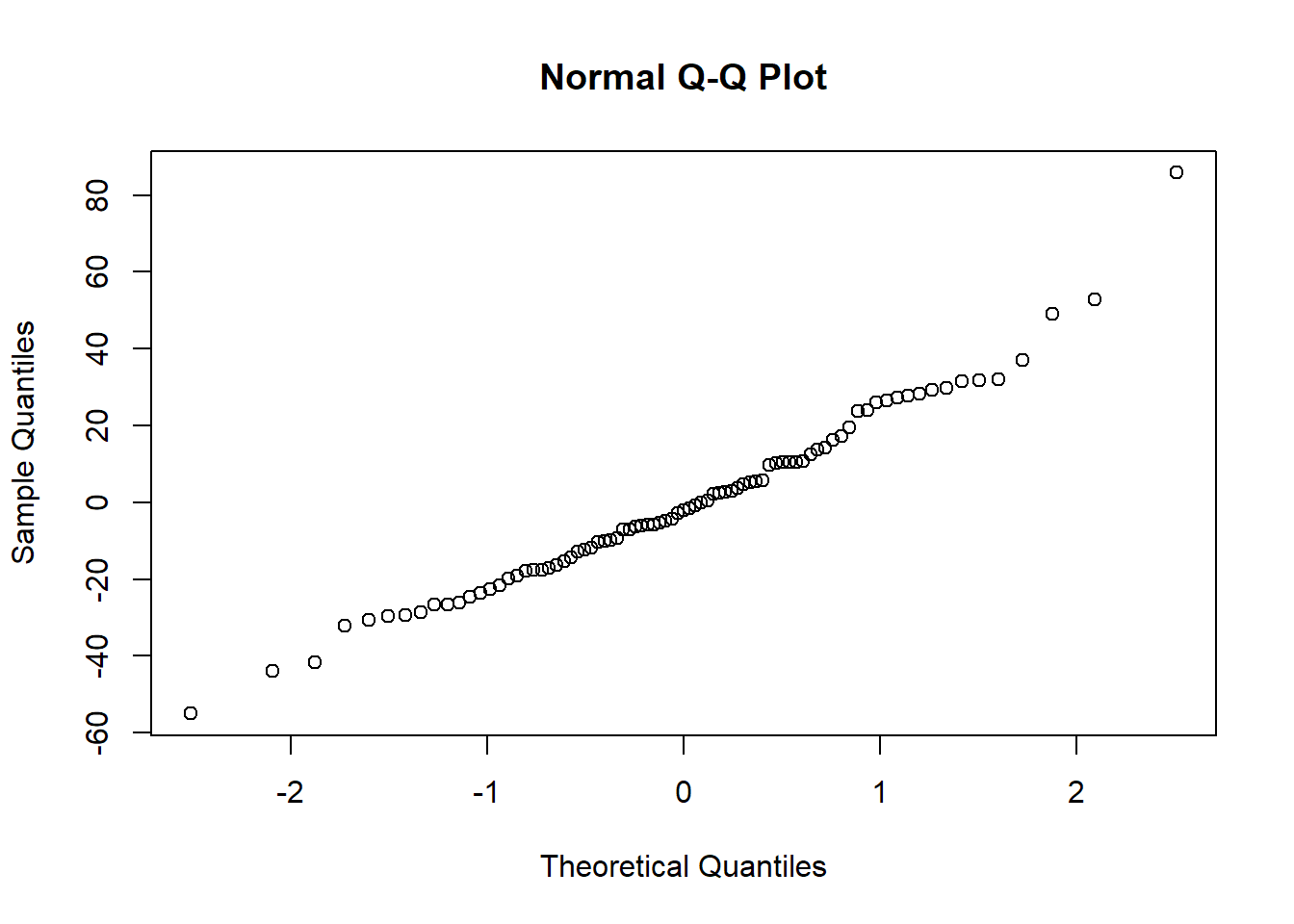
We’re now at the end. There’s a tremendous amount of information and tools for LMMs out there but I’ve put together some of the better introductory ones below. In a future post I’ll cover some more topics re: generalized linear mixed models from lme4 and other libraries.
References, Sources, and Additional Research:
- Linear models and linear mixed effects models in R with linguistic applications (p.26)
- Guide to Mixed Models in R Tufts.edu
- Analysis Factor: Difference between nested and crossed factors
- Just Enough R: 3 Level Models with ‘Partially Crossed’ Random Effects
- Manipulating and summarizing posterior simulations usingrandom variable objects
- Linear Mixed Effects Analysis
- Vignette for
lme4Package - Vignette:
merTools - Wikipedia: Random Effects Model
- GLMMs: Worked Examples
lme4Manual 2010- University of Wisconsin: Madison: Social Science Computing Cooperative
- A Language, not a Letter: Learning Statistics in R
- A brief introduction to mixed effects modelling and multi-model inference in ecology