Fraudulent Transaction Detection with GBM
Introduction
In this post I will be creating a predictive model to identify fraudulent credit card transactions on a public data set from kaggle. Along the way, I will be reviewing some of the functionality of R’s gbm package for predictive modelling.
Data Overview
The data set contiains 280K+ records of credit card transactions from a two-week period in which a small percentage of transactions have been labeled as fraudulent. This data contains 31 columns (features) of which 28 are unnamed and pre-normalized in order to make their contents anonymous.
Gradient Boosting
To identify the fraudulent transactions, I will be using a prediction model in R using the gbm (Gradient Boosted Machines) package.
If you’re not familiar, gradient boosting is a machine learning technique for regression and classification that produces a prediction model in the form of an ensemble of weak prediction models, similar to the random Forrest model I employed in this post. A UC Business Analytics post describes the difference well:
Whereas random forests build an ensemble of deep independent trees, GBMs build an ensemble of shallow and weak successive trees with each tree learning and improving on the previous.
Let’s get started!
library(tidyverse)     # Data wrangling
library(gbm)           # Predictive modelling
library(pROC)          # Model evaluation
library(kableExtra)    # Table formatting
Data & Summary
First we download the compressed data files (3 of them in total) from my general github repo, uncompress them, and combine them into a single file called ccdat. This file contains over 280K records so it may take some time.
mult_zip <- function(baseurl, s){
  # function for downloading multiple gzip files
  # from a github URL where s = seq(start,end)
  ccdat <- data_frame()
  for (i in s){
    daturl = paste0(baseurl, as.character(i), ".csv.gz")
    tmp = tempfile()
    download.file(daturl, tmp)
    df = read.csv(gzfile(tmp))
    ccdat = rbind(ccdat, df)
  }
  return(ccdat)
}
ccurl = paste0("https://raw.githubusercontent.com/jbrnbrg/",
                 "msda-datasets/master/ccdat0")
ccdat <- mult_zip(ccurl, 0:2) %>%
  select(-X)
## Warning: `data_frame()` was deprecated in tibble 1.1.0.
## Please use `tibble()` instead.Next we’ll take a quick look at the data using glimpse - not all the V features are shown as they’re pre-normalized and not very enlightening in this summary view:
ccdat %>%
  select(colnames(ccdat)[c(1:5,20:ncol(ccdat))]) %>%
  glimpse(width = 50)
## Rows: 284,807
## Columns: 17
## $ Time <dbl> 0, 0, 1, 1, 2, 2, 4, 7, 7, 9, 10,~
## $ V1 <dbl> -1.3598071, 1.1918571, -1.3583541~
## $ V2 <dbl> -0.07278117, 0.26615071, -1.34016~
## $ V3 <dbl> 2.53634674, 0.16648011, 1.7732093~
## $ V4 <dbl> 1.37815522, 0.44815408, 0.3797795~
## $ V19 <dbl> 0.40399296, -0.14578304, -2.26185~
## $ V20 <dbl> 0.25141210, -0.06908314, 0.524979~
## $ V21 <dbl> -0.018306778, -0.225775248, 0.247~
## $ V22 <dbl> 0.277837576, -0.638671953, 0.7716~
## $ V23 <dbl> -0.110473910, 0.101288021, 0.9094~
## $ V24 <dbl> 0.06692807, -0.33984648, -0.68928~
## $ V25 <dbl> 0.12853936, 0.16717040, -0.327641~
## $ V26 <dbl> -0.18911484, 0.12589453, -0.13909~
## $ V27 <dbl> 0.133558377, -0.008983099, -0.055~
## $ V28 <dbl> -0.021053053, 0.014724169, -0.059~
## $ Amount <dbl> 149.62, 2.69, 378.66, 123.50, 69.~
## $ Class <int> 0, 0, 0, 0, 0, 0, 0, 0, 0, 0, 0, ~Above, we can see that the only named features are Time, Amount, and Class.
Below, a tabular preview; again, not all the variables are shown.
| Time | V1 | V2 | V3 | V4 | V5 | V6 | V7 | V8 | V9 |
|---|---|---|---|---|---|---|---|---|---|
| 0 | -1.3598071 | -0.0727812 | 2.5363467 | 1.3781552 | -0.3383208 | 0.4623878 | 0.2395986 | 0.0986979 | 0.3637870 |
| 0 | 1.1918571 | 0.2661507 | 0.1664801 | 0.4481541 | 0.0600176 | -0.0823608 | -0.0788030 | 0.0851017 | -0.2554251 |
| 1 | -1.3583541 | -1.3401631 | 1.7732093 | 0.3797796 | -0.5031981 | 1.8004994 | 0.7914610 | 0.2476758 | -1.5146543 |
| 1 | -0.9662717 | -0.1852260 | 1.7929933 | -0.8632913 | -0.0103089 | 1.2472032 | 0.2376089 | 0.3774359 | -1.3870241 |
Feature Review
As previously stated, there are 31 features in this dataset but only Time, Amount, and Class are named. The Class variable identifies the type of transaction (0 for legit, 1 for fraudulent) and is our target variable, Amount is the currency amount of the transaction, and Time is the seconds elapsed between each transaction and the first transaction. Per the data description, the remaining 28 features have been provided post-transformation:
Features V1, V2, … V28 are the principal components obtained with PCA….
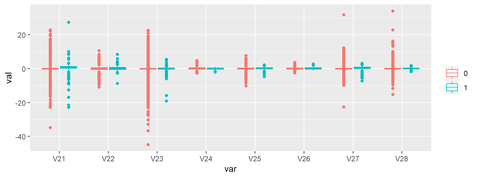
Since there’s a decent number of features and I’m not given any information regarding what the features are or what they contain, I’ll create side-by-side box plots that are separated by Class to give me a quick overview of the differences between legit (Red) and fraudulent (Blue) transaction classes:
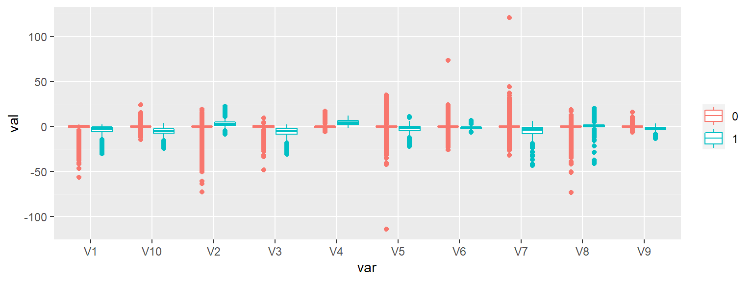
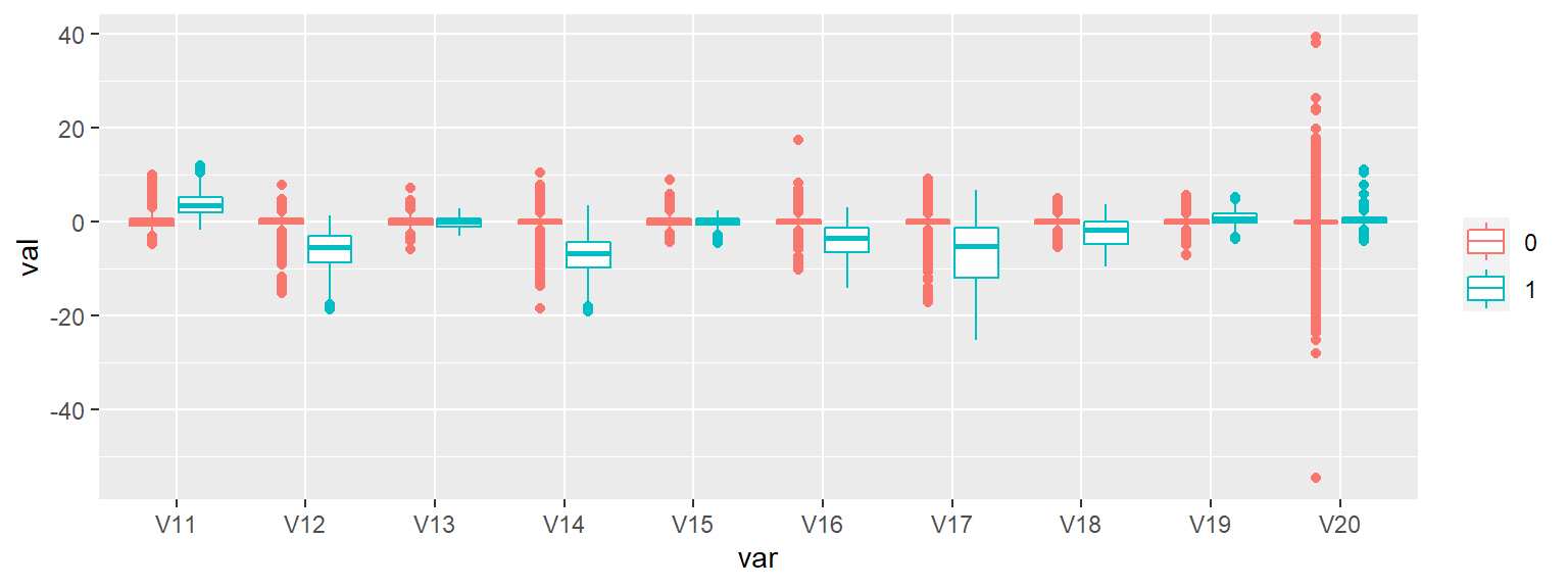
There are a number of features that appear to provide good separation between the fraudulent and legit transactions (e.g. v11, V12, v14, & V17) but looks can be deceiving - I’ll know better after I fit the model and review the feature importance measures.
Train & Test Split
I will be using a 66%/33% split for model training and testing.
tr_te <- sample(c(0,1), nrow(ccdat),
                replace = T,
                prob = c(0.66, 0.33))
train <- ccdat[tr_te == 0,]
test <- ccdat[tr_te == 1,]
Gradient Boosted Model
For a logistic regression, gbm will automatically assume a bernoulli distribution for binary target variables - convenient! There are tons of options not shown in the code chunk below that are also available and the documentation is very good and worth a read.
system.time(
    my_gbm <- gbm(Class ~ .,
                  distribution = 'bernoulli',
                  data = train,
                  n.trees = 300,             # or number of iters
                  interaction.depth = 3,     # max depth of each tree
                  n.minobsinnode = 100,      # min number of obs in nodes
                  shrinkage = 0.01,          # the learning rate
                  bag.fraction = 0.5,        # fraction of training
                  train.fraction = 1)
    )
## user system elapsed
## 97.63 0.09 97.72While certainly not the fasted run time, it’s important to note that the gbm module does perform training and testing of the labeled data.
Feature Importance Review
Below, the summary computes the relative influence of each variable in the gbm model - I’m showing just the top 10 to keep things neat:
feat_importance <- summary(my_gbm, plotit = F)
feat_importance %>% head(10)
## var rel.inf
## V12 V12 31.5554169
## V14 V14 28.8967653
## V17 V17 25.9827440
## V10 V10 5.0675057
## V20 V20 4.3388632
## V7 V7 1.4728345
## V1 V1 0.6891196
## V11 V11 0.6534464
## V4 V4 0.4352978
## V9 V9 0.3512785Model Evaluation
Given the very small number of fraudulent transactions compared to real transactions in this data, I’ll be measuring the accuracy using the Area Under the Curve (Precision/Recall Curve, that is).
test_gbm = predict(my_gbm, newdata = test, n.trees = 300)
gbm_auc = roc(test$Class, test_gbm, plot = TRUE, col = "red")
## Setting levels: control = 0, case = 1## Setting direction: controls < cases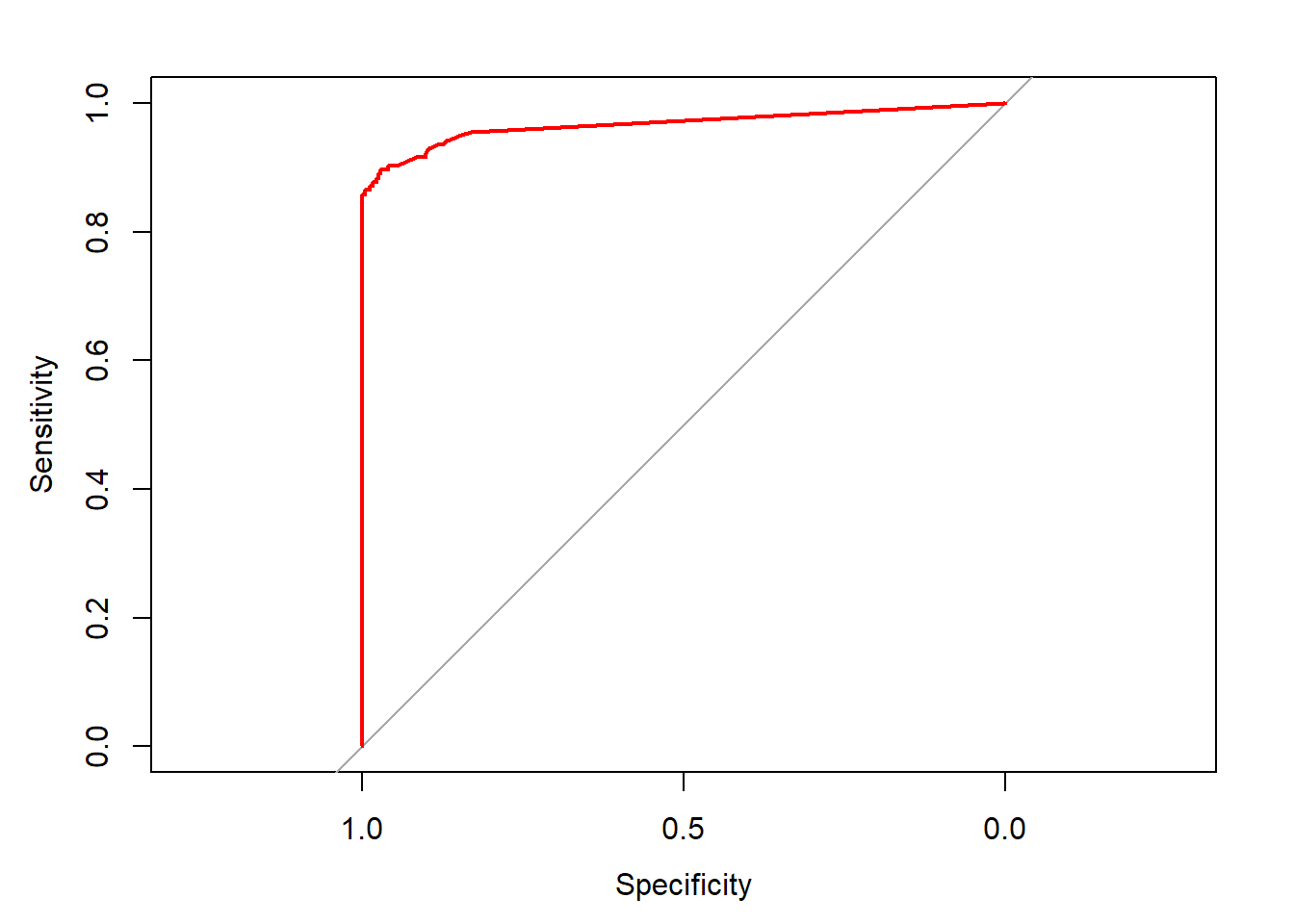
gbm_auc##
## Call:
## roc.default(response = test$Class, predictor = test_gbm, plot = TRUE, col = "red")
##
## Data: test_gbm in 94917 controls (test$Class 0) < 155 cases (test$Class 1).
## Area under the curve: 0.9669While I believe there’s room for improvement, an AUC of ~.93 is pretty good for a basic demonstration of the power of gradient boosting machines on this data. Note that one can get a big performance boost through variable normalization but since this data came with that work already complete, it wasn’t necessary here.