Equity and 311 Heat & Hot Water Service Requests
In this post I’ll be investigating equity between different census tracts in NYC based on economic measures and the open-to-close service request (SR) duration for 311 heat/hot water complaints.
Census Tract Granularity
If you’ve checked out my previous posts, you know I’ve done a bunch of work with NYC’s OpenData at the ZIP-code level. Today I’m going to go a step further and obtain NYC data with latitude and longitude coordinates and merge it with census data by census tract from the 5-year American Community Survey (ACS) from 2016.
While ACS data is available at the ZIP-code level (see zcta) and I’ve used it several times, ZIP codes can span many census tracts. Using the census-tract level provides more detail regarding the socio-economic differences between geographic locations that can be obscured at the ZIP-code level.
311 Service Request Data
The data under investigation will be 311 Service Requests from 2010 to Present – specifically service requests related to complaints about heat and hot water – from NYC’s OpenData platform along with the 5-year American Community Survey data via the very-helpful tidycensus package.
library(lubridate)
library(sf)
library(tidycensus)
library(tidyverse)
library(tigris)
library(RCurl)
library(cowplot)
First I used tidycensus to obtain the ACS data for selected dimensions. You’ll need a census API key that can be obtained here.
census_api_key(Sys.getenv("CENSUS_API_KEY"))
bcodes <- c("005","047", "061", "081", "085")

vars <- c("B01001_001", "B19001_001", "B19083_001", "B19013_001")

nyc <- get_acs(geography = "tract",
               year = 2016,
               variables = vars,
               state = "NY",
               county = bcodes,
               cb = FALSE) %>%
  select(-c("moe")) %>%
  spread(variable, estimate) %>%
  select(ct = GEOID, ct_pop = "B01001_001",
         ct_house_qty = "B19001_001",
         ct_gini = "B19083_001",
         ct_med_inc = "B19013_001")
# Getting data from the 2012-2016 5-year ACS
nyc %>% glimpse()## Rows: 2,167
## Columns: 5
## $ ct <chr> "36005000100", "36005000200", "36005000400", "36005001600~
## $ ct_pop <dbl> 7503, 5251, 5980, 6056, 2682, 9131, 4824, 123, 5651, 3034~
## $ ct_house_qty <dbl> 0, 1331, 1926, 1970, 962, 3008, 1960, 26, 1817, 1076, 143~
## $ ct_gini <dbl> NA, 0.4021, 0.3636, 0.4343, 0.4626, 0.5349, 0.4790, NA, 0~
## $ ct_med_inc <dbl> NA, 70893, 76667, 31540, 39130, 17083, 16503, NA, 21060, ~Below I create a couple of functions for dealing with the json response from the OpenData API and pull down the data:
api_date <- function(y1, m1, d1, y2, m2, d2){
  # start and end date range for API query
  ds = as.Date(paste(toString(y1), toString(m1), d1, sep="-"))
  de = as.Date(paste(toString(y2), toString(m2), d2, sep="-"))
  s = format(ds, "%Y-%m-%dT%H:%M:%OS3")
  e = format(ceiling_date(de, "day") - milliseconds(1),
             "%Y-%m-%dT%H:%M:%OS3")
  return(toString(paste("%27", s, "%27 and %27", e, "%27", sep="")))
}

get_data <- function(surl){
  # transform API response to dataframe
  return(jsonlite::fromJSON(gsub(" ","%20", surl)))
}

date_delta <- function(s,e){
  return(as.numeric(e-s, units = "hours"))
}

my311 <- function(complaint, y1, m1, d1, y2, m2, d2, off, limit){
  # format URL for query to NYC EMS API
  svc311 <- paste0("https://data.cityofnewyork.us/",
                   "resource/fhrw-4uyv.json?",
                   "$$app_token=gTSb6ux3TasUiMp2y0hCqxMRT&$")
  lim_url = paste0("&$limit=", formatC(limit, format = "f", digits = 0))
  offset = paste0("&$offset=", formatC(off, format = "f", digits = 0))

  q_url = paste0(svc311,
                 "select=borough,city,agency,complaint_type,incident_zip,",
                 "incident_address as address,",
                 "count(unique_key) AS svc_qty,",
                 "created_date AS op_date,",
                 "closed_date AS cl_date,",
                 "x_coordinate_state_plane as x_sp,",
                 "y_coordinate_state_plane as y_sp&$",
                 "group=borough,city,agency,complaint_type,",
                 "incident_zip,address,x_sp,y_sp,op_date,cl_date&$",
                 "where=created_date between ",
                 api_date(y1, m1, d1, y2, m2, d2)," AND ",
                 "complaint_type",
                 paste0(" in (%27",
                        paste0(complaint, collapse = "%27,%27"),
                        "%27)"),
                 " AND status in (%27Closed%27) AND ",
                 "borough not in (%27Unspecified%27)",
                 "&$order=borough,city,incident_zip,agency,",
                 "complaint_type,op_date,cl_date",
                 lim_url, offset)
  return(get_data(gsub(" ","%20", q_url)))
}

my311_mult <- function(complaint, y1, m1, d1, y2, m2, d2, limit){
  # pull multi-page data from api
  df = data.frame()
  off = 0
  while(TRUE){
    if (nrow(df) == off){
      df = rbind(df, my311(complaint, y1, m1, d1, y2, m2, d2, off, limit))
      off = off + limit
    }else {
      break
    }
  }
  df = df %>%
    mutate(op_date = ymd_hms(op_date),
           cl_date = ymd_hms(cl_date),
           resp_hr = date_delta(op_date, cl_date),
           x_sp = as.numeric(x_sp),
           y_sp = as.numeric(y_sp)
           )
  return(df)
}

complaint = "HEAT/HOT WATER"
limit = 100000

hh311_new <- my311_mult(complaint, 2017, 10, 1, 2018, 5, 31, limit)
hh311_new %>% glimpse(width = 60)
## Rows: 214,110
## Columns: 12
## $ borough <chr> "BRONX", "BRONX", "BRONX", "BRONX",~
## $ city <chr> "BRONX", "BRONX", "BRONX", "BRONX",~
## $ agency <chr> "HPD", "HPD", "HPD", "HPD", "HPD", ~
## $ complaint_type <chr> "HEAT/HOT WATER", "HEAT/HOT WATER",~
## $ incident_zip <chr> "10451", "10451", "10451", "10451",~
## $ address <chr> "750 GRAND CONCOURSE", "900 GRAND C~
## $ svc_qty <chr> "1", "1", "1", "1", "1", "1", "1", ~
## $ op_date <dttm> 2017-10-01 02:11:22, 2017-10-01 10~
## $ cl_date <dttm> 2017-10-02 08:40:00, 2017-10-02 08~
## $ x_sp <dbl> 1005126, 1005760, 1005746, 1006430,~
## $ y_sp <dbl> 239165, 240735, 239805, 239145, 239~
## $ resp_hr <dbl> 30.47722, 22.26056, 40.96778, 53.97~Next I’ve included some functions I created to deal with observations that had missing lat and lon coordinates. I used the bing maps API and you can sign up for an API token here.
get_lat_lon_url <- function(borough, address){
  # query bing maps API for missing lat/lon points
  bing_token <- Sys.getenv("BING_TOKEN")
  base_url = "http://dev.virtualearth.net/REST/v1/Locations/US/NY/-/"
  q_url = paste0(base_url,
                 borough,"/",address,
                 "?&includeNeighborhood=1&o=json&key=",
                 bing_token)
  return(gsub(" ","%20", q_url))
}

get_lat_lon_df <- function(borough, address, surl){
  # translate Bing API response to df
  rslt_qual = c("High")
  if(surl$resourceSets[[1]]$resources[[1]]$confidence %in% rslt_qual){
    lat = surl$resourceSets[[1]]$resources[[1]]$point$coordinates[[1]]
    lon = surl$resourceSets[[1]]$resources[[1]]$point$coordinates[[2]]
    incident_zip = surl$resourceSets[[1]]$resources[[1]]$address$postalCode[1]
  }else{
    lat = 0
    lon = 0
    incident_zip = 0}
  df = data.frame(borough, address, incident_zip, lat, lon,
                    stringsAsFactors = F)
  return(df)
}

get_lat_lon <- function(borough, address){
  # convert json response to data frame
  surl = get_lat_lon_url(borough, address)
  response = jsonlite::read_json(surl)
  df = get_lat_lon_df(borough, address, response)
  return(df)
}

lat_lon_df <- function(df){
  # creates combined df for addresses with missing lat/lon coords
  # only returns items where match via bing API is "good"
  dft = df %>%
    filter(is.na(lat), is.na(lon)) %>%
    group_by(borough, address) %>%
    summarise(t = n())

  frame = data.frame()
  for (i in 1:nrow(dft)){
    tdf = get_lat_lon(dft[i,]$borough, dft[i,]$address)
    frame = rbind(frame, tdf)
  }
  return(frame %>% filter(incident_zip != "0"))
}
Bing maps didn’t find coordinates for all the addresses but I cleared up a few.
# n_missed <- lat_lon_df(hh311)
# n_missed %>% write.csv("NYC17-18heatMissed.csv")
n_missed <- read.csv("NYC17-18heatMissed.csv",
                      colClasses = c(incident_zip = "character"),
                     stringsAsFactors = F) %>%
  select(-X)
n_repaired <- hh311_new %>%
  filter(is.na(x_sp), is.na(y_sp)) %>%  # 41
  select(-c(x_sp,y_sp,incident_zip)) %>%
  merge(n_missed, by.x = c("borough", "address"), all.x = T)
To get the census tract ID for each lat and lon pair, I used the call_geolocator_latlon function from the tigris library and saved it to a local csv file. This can take a while if you’re working
with a lot of points.
df_points <- read.csv("census_tracts_nyc311.csv",
                      colClasses = c(address = "character",
                      ct_tract = "character")) %>%
  select(-X)

df_points %>% glimpse()
## Rows: 48,253
## Columns: 4
## $ address <chr> "89-21 ELMHURST AVENUE", "1711 FULTON STREET", "9511 SHORE RO~
## $ lat <dbl> 40.74742, 40.67934, 40.61637, 40.84346, 40.84196, 40.82459, 4~
## $ lon <dbl> -73.87685, -73.93044, -74.03827, -73.92470, -73.85773, -73.87~
## $ ct_tract <chr> "360810271001002", "360470297002003", "360470054001002", "360~Next I add my cleaned up observations to the data that I originally pulled, normalize any duplicated calls, and drop observations that are longer than 30 days:
df <- hh311_new %>%
  na.omit() %>%
  arrange(op_date) %>%
  mutate(svc_qty = as.numeric(svc_qty),
         # calls at same exact time combined to 1
         svc_qty = ifelse(svc_qty > 1, 1, svc_qty)) %>%
  filter(resp_hr > 0,       # drops 9 records
         resp_hr / 24 < 30  # drops 21 records greater than 30 days
         ) %>%
  inner_join(df_points, by.x = c("address"), all.x = T) %>%
  mutate(ct = substr(ct_tract, start = 1, stop = 11))
## Joining, by = "address"df %>% glimpse()## Rows: 266,734
## Columns: 16
## $ borough <chr> "BROOKLYN", "MANHATTAN", "MANHATTAN", "BROOKLYN", "BRON~
## $ city <chr> "BROOKLYN", "NEW YORK", "NEW YORK", "BROOKLYN", "BRONX"~
## $ agency <chr> "HPD", "HPD", "HPD", "HPD", "HPD", "HPD", "HPD", "HPD",~
## $ complaint_type <chr> "HEAT/HOT WATER", "HEAT/HOT WATER", "HEAT/HOT WATER", "~
## $ incident_zip <chr> "11221", "10031", "10023", "11235", "10451", "10451", "~
## $ address <chr> "591 MADISON STREET", "515 WEST 147 STREET", "23 WEST ~
## $ svc_qty <dbl> 1, 1, 1, 1, 1, 1, 1, 1, 1, 1, 1, 1, 1, 1, 1, 1, 1, 1, 1~
## $ op_date <dttm> 2017-10-01 00:06:02, 2017-10-01 00:07:17, 2017-10-01 0~
## $ cl_date <dttm> 2017-10-04 10:34:31, 2017-10-05 02:07:03, 2017-10-05 0~
## $ x_sp <dbl> 1002578, 998824, 990867, 994351, 1005126, 1005126, 1005~
## $ y_sp <dbl> 189447, 240517, 222426, 149940, 239165, 239165, 239165,~
## $ resp_hr <dbl> 82.47472, 97.99611, 102.00194, 72.61639, 30.47722, 30.4~
## $ lat <dbl> 40.68665, 40.82683, 40.77718, 40.57822, 40.82310, 40.82~
## $ lon <dbl> -73.93391, -73.94734, -73.97611, -73.96364, -73.92457, ~
## $ ct_tract <chr> "360470293003001", "360610233003000", "360610157001000"~
## $ ct <chr> "36047029300", "36061023300", "36061015700", "360470362~Data Exploration
Next I prepare the data for plotting.
inc_levs <- c(0.00,31167.15,61277.16,91387.18,250001.00)
inc_labels <- c("$0K-31K","$32K-61K","$62K-91K","$92K-250K+")

gini_levs <- c(0.1176,0.4136,0.4546,0.4957,0.7408)
gini_labels <- c("0-Q1","Q1-Q2","Q2-Q3", "Q3+")

plot_dat <- df %>%
  merge(nyc, by.x = "ct", all.x = T) %>%
  mutate(op_ym = strftime(op_date, format="%Y-%m"),
         ct_med_inc_4lev = cut(ct_med_inc,
                               breaks = inc_levs,
                               labels = inc_labels),
         ct_med_inc_2lev = cut(ct_med_inc,
                               breaks = c(0.00,31167.15,250001.00),
                               labels = c("$0K-31K","$32K-250K+")),
         ct_gini_quants = cut(ct_gini,
                               breaks = gini_levs,
                               labels = gini_labels),
         ct_gini_q2 = cut(ct_gini,
                          breaks = c(0.1176,0.4136,0.7408),
                          labels = c("0-Q1","Q1-Q3+"))) %>%
  filter(!is.na(ct_med_inc_4lev),op_date > date("2017-10-2"))

theme1 <- theme(axis.title.x=element_blank(),
                axis.text.x=element_blank(),
                legend.title=element_blank(),
                legend.position="top",
                legend.spacing.x = unit(.5,"cm"),
                legend.box.margin    = margin(.01,.01,0,.01, "cm"),
                #  top, right, bottom, and left
                plot.margin = margin(.01,.2,.1,.5, "cm"))

theme2 <- theme(axis.title.x=element_blank(),
                legend.position="none")
SR Volume and Open-to-Close Duration by CT-level Median Incomes
Here we have the raw counts of SRs per income level on top of boxplots for the SR open-to-close duration in hours:
p1 <- plot_dat %>%
  group_by(op_ym, ct_med_inc_4lev) %>%
  summarise(SR_qty = sum(svc_qty)) %>%
  ggplot(aes(x = op_ym, y = SR_qty,
             fill = ct_med_inc_4lev))+
  geom_bar(stat = "identity", position = "dodge",
           alpha = .8)+
  labs(y = "SR Counts")+
  theme1
## `summarise()` has grouped output by 'op_ym'. You can override using the `.groups` argument.p2 <- plot_dat %>%
ggplot(aes(x = op_ym, y = resp_hr, fill = ct_med_inc_4lev))+
geom_boxplot(alpha=.8,
outlier.alpha = .1)+
labs(y = "SR Duration, Hours")+
theme2
plot_grid(p1, p2, align = "v", nrow = 2, rel_heights = c(3/8, 5/8))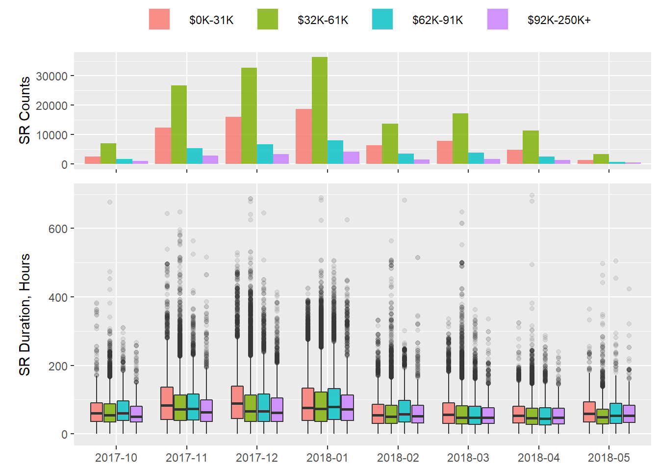
The lower end of the median-income spectrum takes longer than the rest in terms of duration between SR open and close for every month except February 2018.
Combining all median income levels above $0-31K shows a similar pattern:
p3 <- plot_dat %>%
  group_by(op_ym, ct_med_inc_2lev) %>%
  summarise(SR_qty = sum(svc_qty)) %>%
  ggplot(aes(x = op_ym, y = SR_qty,
             fill = ct_med_inc_2lev))+
  geom_bar(stat = "identity", position = "dodge",
           alpha = .8)+
  labs(y = "SR Counts")+
  theme1
## `summarise()` has grouped output by 'op_ym'. You can override using the `.groups` argument.p4 <- plot_dat %>%
ggplot(aes(x = op_ym, y = resp_hr,
fill = ct_med_inc_2lev))+
geom_boxplot(alpha=.8,
outlier.alpha = .1)+
labs(y = "SR Duration, Hours")+
theme2
plot_grid(p3, p4, align = "v", nrow = 2, rel_heights = c(3/8, 5/8))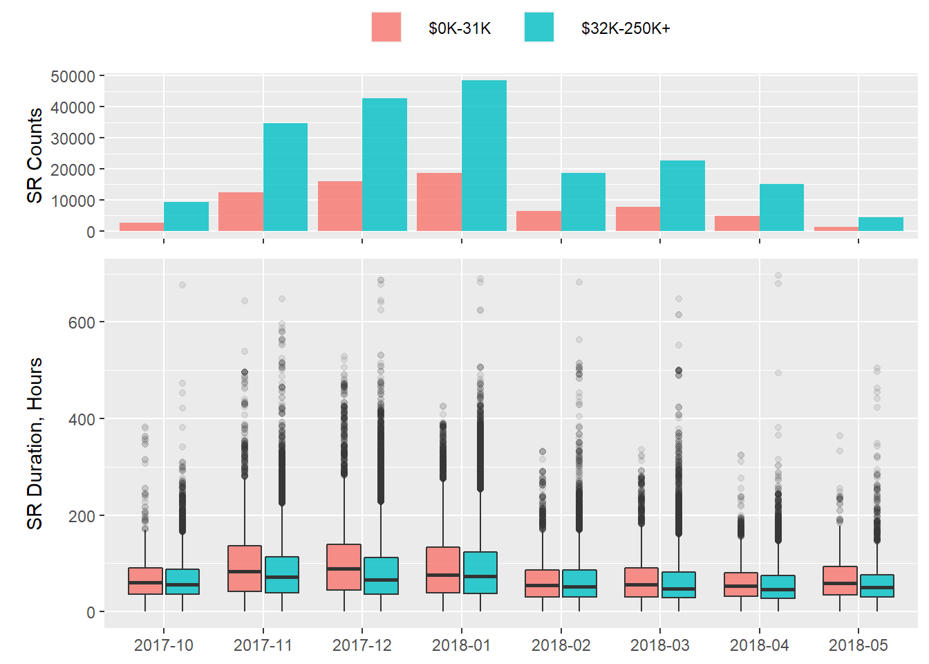
Although the $32K-250K+ median income levels have over double the number of calls per month, they still lag behind with longer SR open-to-close durations.
SR Volume and Open-to-Close Duration by CT-level Gini Coefficients
Next we’ll review the same measures broken down by census tract Gini values. From the Wikipedia article:
The Gini coefficient measures the inequality among values of a frequency distribution (for example, levels of income). A Gini coefficient of zero expresses perfect equality, where all values are the same (for example, where everyone has the same income). A Gini coefficient of 1 (or 100%) expresses maximal inequality among values (e.g., for a large number of people, where only one person has all the income or consumption, and all others have none, the Gini coefficient will be very nearly one).
To give you a sense for NYC’s census tract Gini values, here is a histogram of the values among the 2K+ census tracts in the data:
nyc %>%
  na.omit() %>%
  ggplot(aes(x=ct_gini))+
  geom_histogram(alpha = .8, bins = 50)+
  labs(x= "Gini Coefficient",
       y= "Frequency")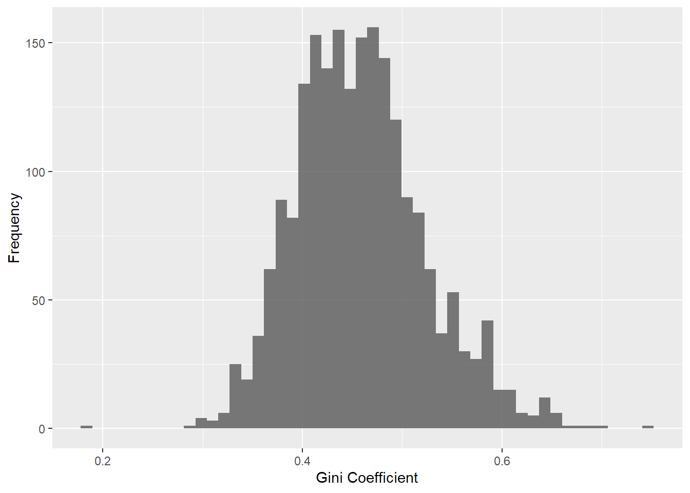
And a summary of the Gini values:
nyc$ct_gini %>% summary()## Min. 1st Qu. Median Mean 3rd Qu. Max. NA's
## 0.1176 0.4136 0.4546 0.4580 0.4957 0.7408 54The following plots are broken into the above quantiles
p5 <- plot_dat %>%
  group_by(op_ym, ct_gini_quants) %>%
  summarise(SR_qty = sum(svc_qty)) %>%
  ggplot(aes(x = op_ym, y = SR_qty,
             fill = ct_gini_quants))+
  geom_bar(stat = "identity", position = "dodge",
           alpha = .8)+
  labs(y = "SR Counts")+
  theme1
## `summarise()` has grouped output by 'op_ym'. You can override using the `.groups` argument.p6 <- plot_dat %>%
ggplot(aes(x = op_ym, y = resp_hr,
fill = ct_gini_quants))+
geom_boxplot(alpha=.8,
outlier.alpha = .1)+
labs(y = "SR Duration, Hours")+
theme2
plot_grid(p5, p6, align = "v", nrow = 2, rel_heights = c(3/8, 5/8))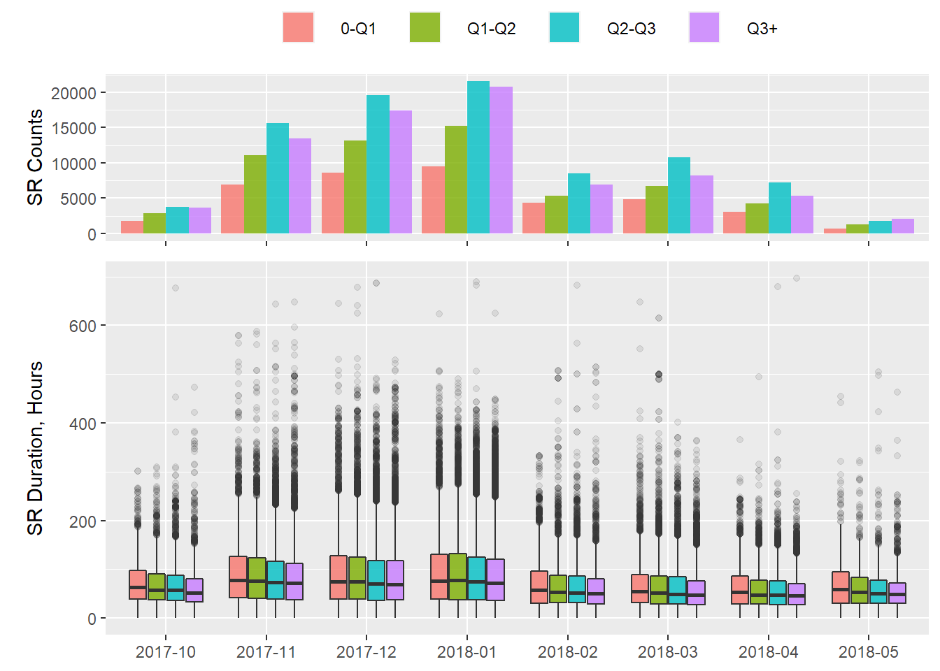
This plot indicates that more income equality (0-Q1) leads to longer SR open-to-close duration while more income inequality (Q3+) leads to shorter SR open-to-close duration.
Next, I’ll compare 0-Q1 with Q1 through Q3+ grouped:
p7 <- plot_dat %>%
  group_by(op_ym, ct_gini_q2) %>%
  summarise(SR_qty = sum(svc_qty)) %>%
  ggplot(aes(x = op_ym, y = SR_qty,
             fill = ct_gini_q2))+
  geom_bar(stat = "identity", position = "dodge",
           alpha = .8)+
  labs(y = "SR Counts")+
  theme1
## `summarise()` has grouped output by 'op_ym'. You can override using the `.groups` argument.p8 <- plot_dat %>%
ggplot(aes(x = op_ym, y = resp_hr,
fill = ct_gini_q2))+
geom_boxplot(alpha=.8,
outlier.alpha = .1)+
labs(y = "SR Duration, Hours")+
theme2
plot_grid(p7, p8, align = "v", nrow = 2, rel_heights = c(3/8, 5/8))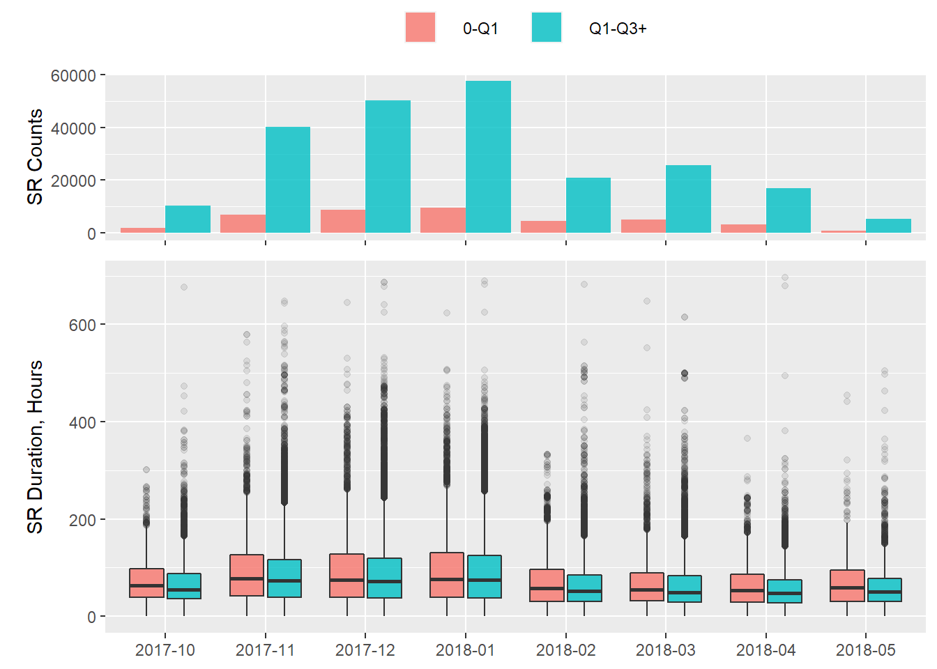
The pattern of longer open-to-close SR duration for census tracts with higher levels of income equality remains.
Scope and Risks
This brief exploration was focused on equity for heat/hot water calls by comparing open-to-close service request SR duration for census tracts of NYC broken down by economic measures.
While this analysis indicates a potential of income-based inequality for heat/hot water service calls, it is not conclusive and should be taken with a grain of salt. Below I have listed the specifics of the data and some important points of consideration:
- SRs under investigation span 2017-2018 heating season (October 1st through May 31st) that have a SR status of closed
- SRs that originate from the same address at the same time have been re-leveled to account for a single calls
- 25 SRs have been removed for lack census-tract available information and 30 SRs were removed for being longer than 30 days or having a duration equal to zero
- SR open-to-close duration is unlikely to comprehensively measure the duration that NYC residents were without heat - there is likely an administrative element related to NYC’s 311 agency related to this duration that could overstate the duration in a number of ways
- Housing units with an owner on-premises may deal with heat & hot water problems differently than multi-tenant apartment buildings
- A 2017 studyfound that there are socio-spatial differentials in the propensity to complain about heat and hot water using 311 (i.e. certain populations under-use –or not use at all – 311 while others use it frequently)
- Older buildings may need more service requests