Structural Time Series Forecasting

Unlike traditional time-series model forecasting, BSTS models can be used for prediction for multiple correlated time series while handling large variations in the short term. The Bayesian part, with respect to multivariate variables, assists the model to avoid over-fitting and identify correlations among the variables.

Because BSTS models allow for the inclusion of multiple seasonal/cyclic exogenous features (i.e. features that impact the model without being affected by it) that are themselves functions of time, it’s a great candidate to help me forecast EMS call volume using historical call volume and historical temperature data.

There’s a lot more to understand about the capabilities of BSTS - see the the References at the bottom of this post for links to further information and resources.

As this library is new and in active development, this post relies on tf’s example post found here that also details how to install tensorflow_probability and provides the code for the plots below.

EMS Call Volume Forecasting with BSTS:

import matplotlib as mpl
import datetime
from matplotlib import pylab as plt
import matplotlib.dates as mdates
import seaborn as sns
import collections
import pandas as pd
import numpy as np
import tensorflow as tf
import tensorflow_probability as tfp
from tensorflow_probability import distributions as tfd
from tensorflow_probability import sts

Next I prep an abridged portion of my EMS data that contains only the CALL_QTY and TEMP features and spans the dates 6/5/2016 through 7/31/2016. Features such as INC_DOW (incident day of week) and INC_H (incident hour of the day) will be handled by the build_model function below.

alldata = pd.read_csv('emsforsts.csv')

Here’s a look at the raw data:

            Unnamed: 0  CALL_QTY  INC_DOW  INC_H  TEMP  DEWP
0  2016-06-05 00:00:00     174.0      0.0    0.0  69.0  67.0
1  2016-06-05 01:00:00     147.0      0.0    1.0  68.0  65.0
2  2016-06-05 02:00:00     122.0      0.0    2.0  66.0  63.0
3  2016-06-05 03:00:00     135.0      0.0    3.0  67.0  64.0
4  2016-06-05 04:00:00     127.0      0.0    4.0  67.0  63.0

Set up the data to be ingested by tensorflow, create the forecast window, and make the training data set:

emsdates = np.array(alldata["Unnamed: 0"], dtype='datetime64[h]')
calls = np.array(alldata.CALL_QTY).astype(np.float32)
temperature = np.array(alldata.TEMP).astype(np.float32)
num_forecast_steps = 24 * 7 * 2 # 2-week forecast
ems_train = calls[:-num_forecast_steps] # training portion

Here’s a quick view of call volume and temperature over time:

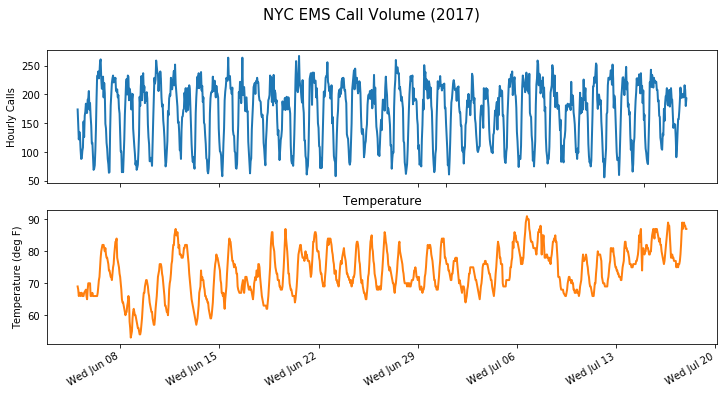
Call Volume and Temperature over time

Next, the build_model function allows me to include some additional exogenous features. Recall the seasonal decomposition of the call volume in this post where I identified the daily and weekly seasonality.

def build_model():
  hour_of_day_effect = sts.Seasonal(num_seasons=24,
                                    observed_time_series=calls,
                                    name='hour_of_day_effect')
  day_of_week_effect = sts.Seasonal(
      num_seasons=7, num_steps_per_season=24,
      observed_time_series=calls,
      name='day_of_week_effect')
  temperature_effect = sts.LinearRegression(
      design_matrix=tf.reshape(temperature - np.mean(temperature),
                               (-1, 1)), name='temperature_effect')
  autoregressive = sts.Autoregressive(
      order=1,
      observed_time_series=calls, name='autoregressive')
  model = sts.Sum([hour_of_day_effect,
                   day_of_week_effect,
                   temperature_effect,
                   autoregressive],
                   observed_time_series=calls)
  return model
tf.reset_default_graph()
ems_model = build_model()

Next I train the model using the variational loss functions and “surrogate posteriors” (see the references at the end of this post for more information):

with tf.variable_scope('sts_elbo', reuse=tf.AUTO_REUSE):
  elbo_loss, variational_posteriors = tfp.sts.build_factored_variational_loss(
      ems_model, ems_train)
train_vi = tf.train.AdamOptimizer(0.1).minimize(elbo_loss)
num_variational_steps = 201
num_variational_steps = int(num_variational_steps)
with tf.Session() as sess:
  sess.run(tf.global_variables_initializer())
  for i in range(num_variational_steps):
    _, elbo_ = sess.run((train_vi, elbo_loss))
    if i % 20 == 0:
      print("step {} -ELBO {}".format(i, elbo_))
  q_samples_calls_ = sess.run({k: q.sample(50)
                                for k, q in variational_posteriors.items()})

The printed output provides the loss at selected steps:

step 0 -ELBO 78367.3984375
step 20 -ELBO 10542.7236328125
step 40 -ELBO 7598.81787109375
step 60 -ELBO 6851.21142578125
step 80 -ELBO 6484.31103515625
step 100 -ELBO 6180.28564453125
step 120 -ELBO 5911.81982421875
step 140 -ELBO 5768.7216796875
step 160 -ELBO 5617.462890625
step 180 -ELBO 5493.638671875
step 200 -ELBO 5398.287109375

I then review the parameters and allows me to see their rough impact on the model:

print("Inferred parameters:")
for param in ems_model.parameters:
  print("{}: {} +- {}".format(param.name,
                              np.mean(q_samples_calls_[param.name], axis=0),
                              np.std(q_samples_calls_[param.name], axis=0)))

Inferred parameters:
observation_noise_scale: 3.97651529 +- 0.0263753459
hour_of_day_effect/_drift_scale: 3.432635307 +- 0.01715491526
day_of_week_effect/_drift_scale: 3.021797419 +- 0.0963104665
temperature_effect/_weights: [-0.24923329] +- [0.0319189]
autoregressive/_coefficients: [0.95459527] +- [0.00140634]
autoregressive/_level_scale: 5.42514611 +- 0.02468751743

Next, I create the forecast with tfp.sts.forecast:

calls_forecast_dist = tfp.sts.forecast(
    model=ems_model,
    observed_time_series=ems_train,
    parameter_samples=q_samples_calls_,
    num_steps_forecast=num_forecast_steps)
num_samples=10
with tf.Session() as sess:
  (calls_forecast_mean,
   calls_forecast_scale,
   calls_forecast_samples) = sess.run(
      (calls_forecast_dist.mean()[..., 0],
       calls_forecast_dist.stddev()[..., 0],
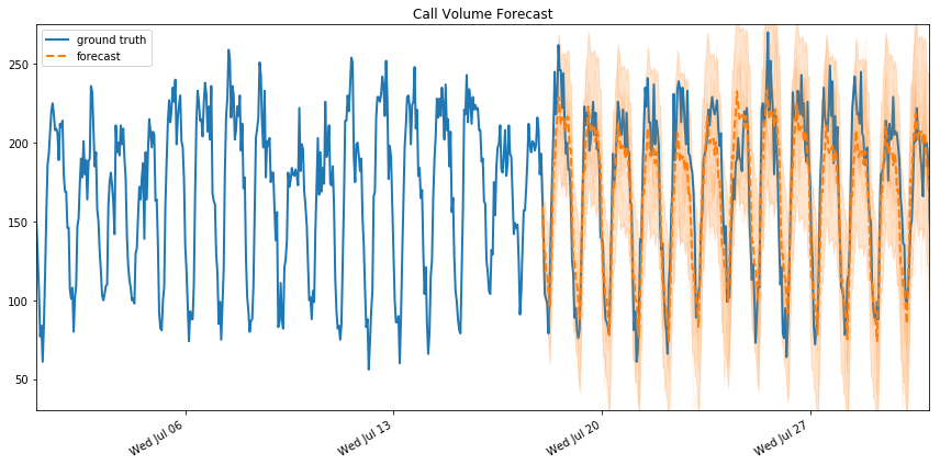
       calls_forecast_dist.sample(num_samples)[..., 0]))

And here’s the plotted forecast along with the actual values - not too shabby:

As mentioned, sts provides the ability visualize the decomposition of the data and forecast into individual parts. First we get the distributions over each output from the “posterior marginals” on both the training and forecast model:

component_dists = sts.decompose_by_component(
    ems_model,
    observed_time_series=ems_train,
    parameter_samples=q_samples_calls_)
forecast_component_dists = sts.decompose_forecast_by_component(
    ems_model,
    forecast_dist=calls_forecast_dist,
    parameter_samples=q_samples_calls_)
with tf.Session() as sess:
  calls_component_means_, calls_component_stddevs_ = sess.run(
      [{k.name: c.mean() for k, c in component_dists.items()},
       {k.name: c.stddev() for k, c in component_dists.items()}])
  [
      calls_forecast_component_means_,
      calls_forecast_component_stddevs_
  ] = sess.run(
      [{k.name: c.mean() for k, c in forecast_component_dists.items()},
       {k.name: c.stddev() for k, c in forecast_component_dists.items()}])

# Combine training with forecast data for plot
component_with_forecast_means_ = collections.OrderedDict()
component_with_forecast_stddevs_ = collections.OrderedDict()
for k in calls_component_means_.keys():
  component_with_forecast_means_[k] = np.concatenate([
      calls_component_means_[k],
      calls_forecast_component_means_[k]], axis=-1)
  component_with_forecast_stddevs_[k] = np.concatenate([
      calls_component_stddevs_[k],
      calls_forecast_component_stddevs_[k]], axis=-1)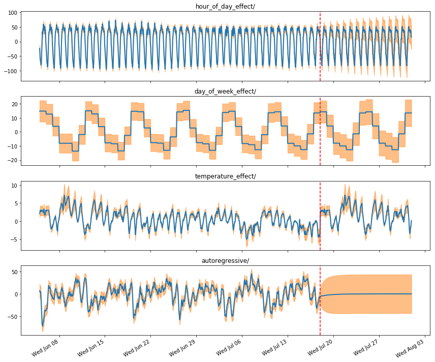

Model Decomp

Above, the red dotted line indicates where the forecast begins.

Next, I’ll make a simple anomaly detection scheme to tag all time steps where the observations are more than 3 standard deviations from the predicted value. These are the time steps where model was most “surprised.” To complete this, I’ll use the forecast for each hour, given only the hours up to that point.

# one-step predictive distributions:
demand_one_step_dist = sts.one_step_predictive(
    ems_model,
    observed_time_series=calls,
    parameter_samples=q_samples_calls_)
with tf.Session() as sess:
  calls_one_step_mean = sess.run(demand_one_step_dist.mean())
  calls_one_step_scale = sess.run(demand_one_step_dist.stddev())
fig, ax = plot_one_step_predictive(
    emsdates, calls,
    calls_one_step_mean, calls_one_step_scale,
    x_locator=ems_loc, x_formatter=ems_fmt)
ax.set_ylim(30, 275)
zscores = np.abs((calls - calls_one_step_mean) /
                 calls_one_step_scale)
anomalies = zscores > 3.0
ax.scatter(emsdates[anomalies],
           calls[anomalies],
           c="red", marker="x", s=15, linewidth=2, label="Anomalies (>3$\sigma$)")
ax.plot(emsdates, zscores, color="black", alpha=0.1, label='predictive z-score')
ax.legend()

Here is the resulting plot:

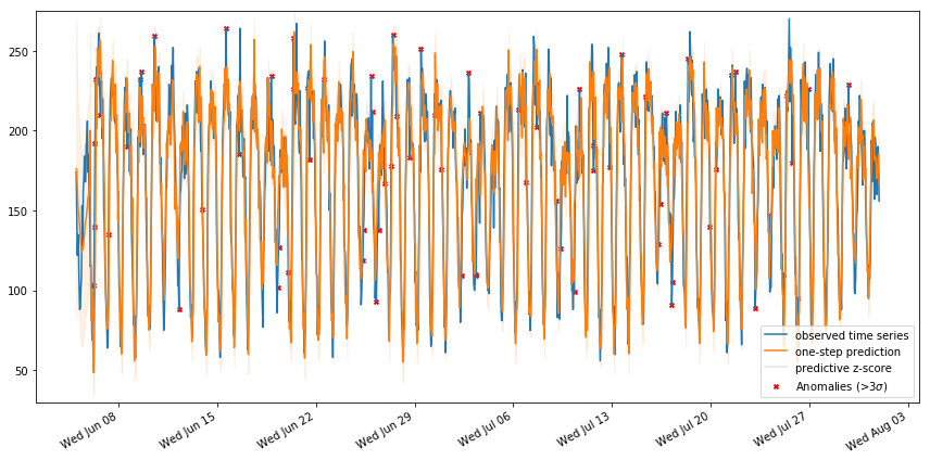
Forecast Anomoly Review

As shown above, there are a lot of anomalies to consider but this is just a simple demonstration of the sts package so I’ll leave it as is.

Finally, let’s take a look at the rmse:

np.sqrt(((calls_one_step_mean - calls) ** 2).mean())
# 19.84311

While I’ve achieved superior scores using LSTM, this model is far more interpret-able than an LSTM which is a tremendous advantage in the business world.

Tensorflow’s BSTS method is a powerful option for multi-variate seasonal time series forecasting and I highly recommend checking it out.

References:

• Multivariate Bayesian Structural Time Series Model
• Tensorflow Probabilty
• Wikipedia: Baysian Structural Time Series
• Forecasting with Structural Time Series Models
• Variational Inference - Princeton CS
• Variational Inference - Deriving the ELBO
• ELBO Gradient Estimators: pyro.ai documentation