Traditional forecasting methods require stationary data to make a valid forecast. In this post I’ll run through a relatively simple time-series forecast that employs forcast package’s auto.arima function and regression tress to via the rpart library.

library(RCurl)
library(forecast)
library(lubridate)
library(tidyverse)
library(ggforce)
library(kableExtra)
library(rpart)
library(rpart.plot)
library(data.table)

Here’s a preview of the data I’m working with. It’s the same EMS data (with different aggregations) from my EMS Flexdashboard post. https://jbrnbrg.github.io/post/nyc-ems-flexdashboard-plotly/

INC_DAYH	AVG_DISP_SEC	AVG_TRAV_SEC	CALL_QTY	INC_DOW	INC_H	INC_YMD	INC_WOY	INC_Y
2013-01-01 00:00:00	379.3090	447.0037	288	2	0	2013-01-01	1	2013
2013-01-01 01:00:00	993.4384	457.8976	333	2	1	2013-01-01	1	2013
2013-01-01 02:00:00	1147.9193	628.4567	384	2	2	2013-01-01	1	2013
2013-01-01 03:00:00	1171.4780	517.7113	318	2	3	2013-01-01	1	2013
2013-01-01 04:00:00	818.1272	498.5076	283	2	4	2013-01-01	1	2013
2013-01-01 05:00:00	608.9864	500.8824	220	2	5	2013-01-01	1	2013

First I preview the data to note the seasonality of the call quantities over the years:

ems %>% group_by(INC_YMD) %>% 
  summarise(CALL_QTY = sum(CALL_QTY)) %>%
  ggplot(aes(x = INC_YMD, y = CALL_QTY)) +
  geom_line()+
  facet_zoom(x = (INC_YMD %in% tail(unique(ems$INC_YMD), 24*7*3)), 
             zoom.size = 1.5)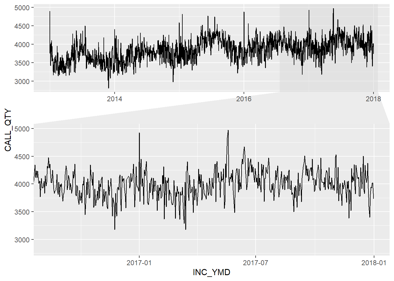

Zooming into 3 weeks reveals additional seasonality that will also need to be dealt with.

First I’ll break up the full data into 3 weeks + one day for use in testing and training. Then I’ll employ the msts function from the forecast library to decompose the seasons and reveal the underlying trend.

# 3 weeks + 1 day depicting the train/testing data
e <- ems %>% 
  filter(INC_YMD >= ymd("2013-1-1") & INC_YMD < ymd("2013-1-23"))

# create test and training sets. 
d_spine <- seq(head(e$INC_DAYH, 1), 
               tail(e$INC_DAYH, 1), 
               by="hour")

etrain <- e %>% # 3 weeks total 
  filter(INC_DAYH %in% 
           d_spine[1:(length(d_spine)-24)])
etest <- ems %>% # 24 hours 
  filter(INC_DAYH %in% 
           d_spine[(length(d_spine)-24 + 1):(length(d_spine))])

Below, the trend has been revealed and even though the Remainder still indicates some seasonality that’s not dealt with, I will forge ahead.

calls_msts <- msts(etrain$CALL_QTY, seasonal.periods = c(24, 7*24))

calls_msts %>% mstl() %>% autoplot()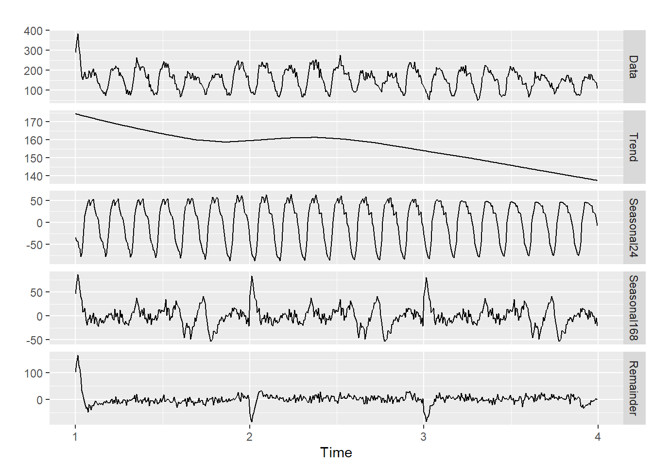

I’ll now fit an auto.arima() model to the Trend part and review the prediction.

# break into: trend, season24, season24x7, remainder
decomp_call <- calls_msts %>% mstl()

# fit trend portion via auto.arima
calls_trend_fit <- auto.arima(decomp_call[, 'Trend'], lambda = 0)

# forecast 1 period (24hours) ahead using the mean of the fit
calls_fcst <- forecast(calls_trend_fit, 24)$mean

Visual representation of the foretasted trend-portion of the calls:

# visualize the forecasted trend portion with actual. 
trend_fcst_df <- data.table(call_qty = c(decomp_call[, 'Trend'], 
                                         calls_fcst), 
                            date_col = c(etrain$INC_DAYH, etest$INC_DAYH), 
                            data_type = c(rep("Actual", 
                                              length(decomp_call[, 'Trend'])),
                                          rep("Forecast", length(calls_fcst))))

ggplot(trend_fcst_df, aes(date_col, call_qty, color = data_type)) +
  geom_line(size = 1.2) +
  labs(title = paste(calls_trend_fit))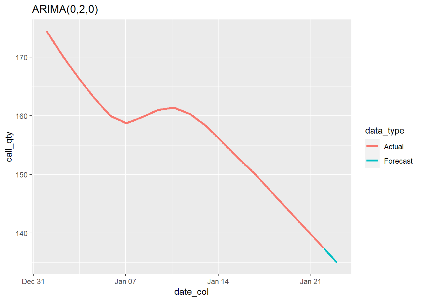

But what about the seasonal portion? Here, I’ll employ the fourier function and use the rpart’s regression tress for forecasting. The Fourier components allow me to model the seasonality and will be included in the features of the model.

N <- length(etrain$CALL_QTY)
w <- (N / 24) - 1                     # days in the training 
                                      # with 24hrs lag
calls_detrended <- rowSums(decomp_call[, c(3,4,5)]) 
                                      # add "seasonal" and "remainder"
                                      # to form detrended data
                                      # this part will be predicted using Rpart
                                      # and the trend will be predicted using ARIMA

fourierParts <- fourier(msts(etrain$CALL_QTY,
                             seasonal.periods = c(24)),
                        K=c(2))

lagems <- rowSums(decomp_call[1:(w*24),c(3,4)]) # first to 20 days

lil_train <- data.table(Calls = tail(calls_detrended,w*24), # last 20 days
                        fourierParts[(24+1):N,],            # last 20 days
                        l_calls = lagems                    # first 20 days
                        )

mape <- function(real, pred){
  # MAPE - Mean Absolute Percentage Error
  return(100 * mean(abs((real - pred)/real))) 
}

Here’s a view of the data:

Calls	S1-24	C1-24	S2-24	C2-24	l_calls
-58.99558	0.2588190	0.9659258	0.5000000	0.8660254	11.583955
-71.85072	0.5000000	0.8660254	0.8660254	0.5000000	23.942616
-74.70585	0.7071068	0.7071068	1.0000000	0.0000000	43.460696
-85.56099	0.8660254	0.5000000	0.8660254	-0.5000000	16.531488
-80.41612	0.9659258	0.2588190	0.5000000	-0.8660254	-4.572146
-95.27126	1.0000000	0.0000000	0.0000000	-1.0000000	-36.881419

Now I train the model and review the decision tree created by rpart. Not that the SX-Y and CX-Y variables represent the Fourier pairs for the seasonal parts.

t1 <- rpart(Calls ~ ., data = lil_train)
#t1$variable.importance
#t1 %>% summary()
rpart.plot(t1, digits = 2)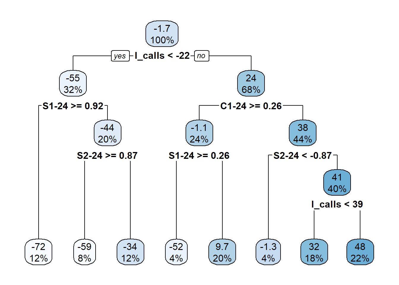

The plot indicates that the one-day lagged calls is the most important feature followed by the the 24 hour portion of the Fourier features.

Next I’ll try out a simple forecast to see how it does:

datas <- data.table(Calls = c(lil_train$Calls,
                             predict(t1)),
                    Time = rep(1:length(lil_train$Calls), 2),
                    Type = rep(c("Real", "RPART"), 
                               each = length(lil_train$Calls)))
ggplot(datas, aes(Time, Calls, color = Type)) +
  geom_line(size = 0.8, alpha = 0.75) +
  labs(y = "Calls (detrended)", title = "Fitted values from RPART tree")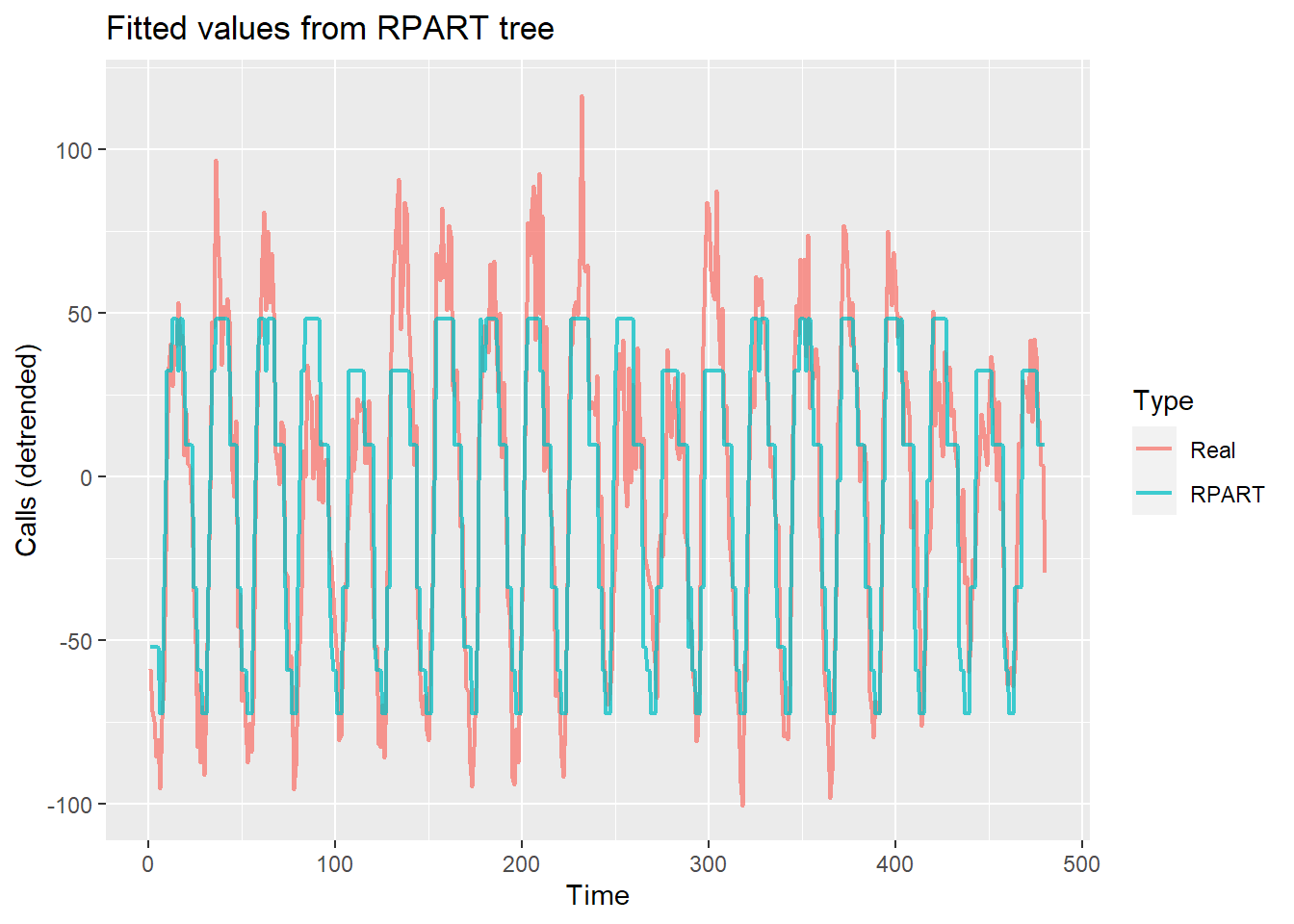

It certainly doesn’t look great - it’s been chopped at all of the peaks. Here’s the mape:

mape(lil_train$Calls, predict(t1))

## [1] 348.5485

This is not a wonderful score but it can be improved. This will be done by adding control for the rpart fit. The parameter cp or “complexity parameter” is best explained in the help menu from rpart.control:

> Any split that does not decrease the overall lack of fit by a factor of cp is not attempted. For instance, with anova splitting, this means that the overall R-squared must increase by cp at each step. The main role of this parameter is to save computing time by pruning off splits that are obviously not worthwhile. Essentially,the user informs the program that any split which does not improve the fit by cp will likely be pruned off by cross-validation, and that hence the program need not pursue it.

Further, a minsplit of 2 ensures that at least two observations must exist in a tree node in order for the split to be attempted. Using a maxdepth of 30 gives my tree plenty of room to grow from the first node which is at a depth of 0.

t2 <- rpart(Calls ~ ., data = lil_train,
            control = rpart.control(minsplit = 2,
                                    maxdepth = 30,
                                    cp = 0.000001))
datasx <- data.table(Calls = c(lil_train$Calls,
                             predict(t2)),
                    Time = rep(1:length(lil_train$Calls), 2),
                    Type = rep(c("RPART", "real"), 
                               each = length(lil_train$Calls)))
ggplot(datasx, aes(Time, Calls, color = Type)) +
  geom_line(size = 0.8, alpha = 0.75) +
  labs(y = "Calls (detrended)", 
       title = "Fitted values from RPART tree")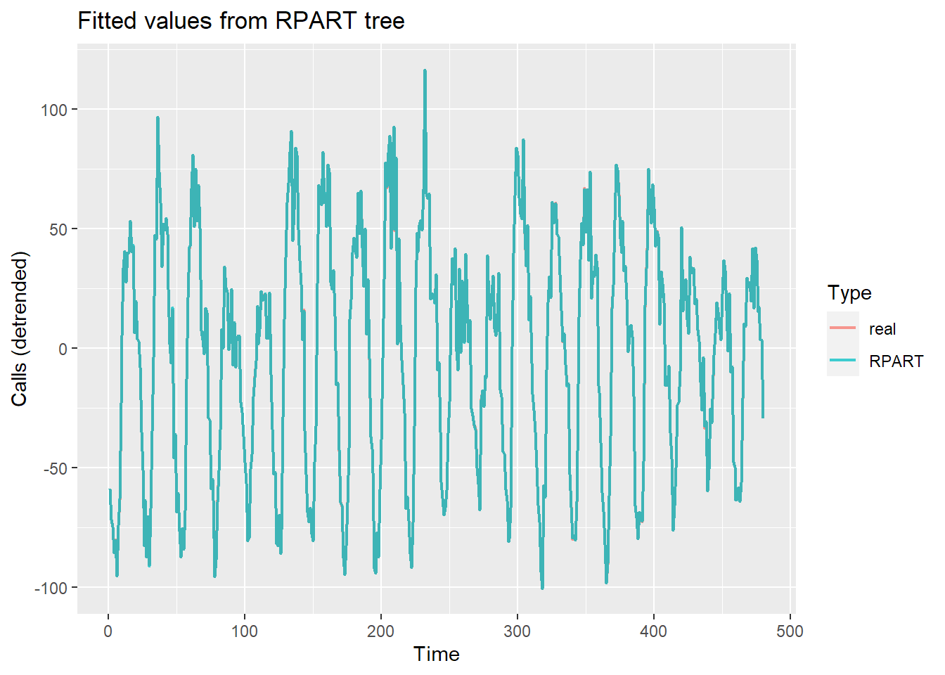

This certainly looks better - I can barely make out the real portion. It may look good but it’s possible that I’ve over-fit. Here’s the mape:

mape(lil_train$Calls, predict(t2))

## [1] 0.2463635

This is still an improvement so pushing ahead I’ll test out the model. I do this by combining the auto.arima forecast of the trend and the rpart regression trees for the seasonal part:

lagems_test <- rowSums(decomp_call[(w*24+1):N,c(3,4)])
fourierParts_test <- fourier(msts(etrain$CALL_QTY,
                                  seasonal.periods = c(24)),
                             K=c(2), h = 24) # h results in forecast ahead
lil_test <- data.table(fourierParts_test, 
                       l_calls = lagems_test)

# add in the ARIMA trend portion 
pred24 <- predict(t2, lil_test) + calls_fcst

dfor <- data.table(Calls = c(etrain$CALL_QTY, 
                             etest$CALL_QTY, 
                             pred24),
                   Date = c(etrain$INC_DAYH,
                            rep(etest$INC_DAYH, 2)),
                   Type = c(rep("Train data", length(etrain$INC_DAYH)),
                            rep("Test data", nrow(etest)),
                            rep("Forecast", nrow(etest))))

ggplot(dfor, aes(Date, Calls, color = Type)) +
  geom_line(size = 0.8, alpha = 0.75) +
  facet_zoom(x = Date %in% tail(dfor$Date,60), 
             zoom.size = 1.5) +
  labs(title = "Forecast from RPART")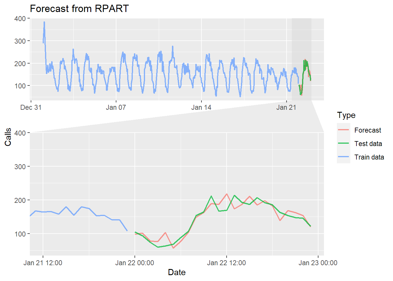

The forecast appears to fit well. Additional diagnostics will be required to confirm this as well as some cross validation vs a naive forecast that repeats the previous 24 hour period.