In today’s post I build upon the last post to demonstrate the use of the tmap package to make a choropleth map in R. I also include instructions on how to use the sf library to obtain the block-level census tract IDs included in the tidycensus ACS data for the State Plane coordinates within the NYC 311 data.

If you’re new to making maps, it’s important that you recognize the differences between geographic coordinate and projected coordinate systems. Although many data sources provide both (e.g. latitude/longitude and state plane x/y) and many mapping libraries can work with both, not all functions within libraries will work with both and conversion will be needed (e.g. sf provides the st_transform function that uses GDAL for coordinate transformation).

Let’s get started!

library(tidyverse)     # wrangling
library(tidycensus)    # nyc shape files and economic data
library(lubridate)     # date conversion
library(tigris)        # area_water
library(sf)            # joining by geographical data
library(tmap)          # chorpleths
library(RColorBrewer)  # palettes
options(tigris_use_cache = TRUE)

# Other libraries referenced: 
# lwgeom::             # for repairing geometries
# jsonlite::           # converting json to df

Like last time, we pull the data from NYC’s OpenData API but unlike the last post, we pull out the x/y_coordinate_state_plane fields as these coordinates are necessary for the st_join that’s coming up later.

api_date <- function(y1, m1, d1, y2, m2, d2){
  # start and end date range for API query
  ds = as.Date(paste(toString(y1), toString(m1), d1, sep="-"))
  de = as.Date(paste(toString(y2), toString(m2), d2, sep="-"))
  s = format(ds, "%Y-%m-%dT%H:%M:%OS3")
  e = format(ceiling_date(de, "day") - milliseconds(1), 
             "%Y-%m-%dT%H:%M:%OS3")
  return(toString(paste("%27", s, "%27 and %27", e, "%27", sep="")))
}

get_data <- function(surl){
  # transform API response to dataframe
  return(jsonlite::fromJSON(gsub(" ","%20", surl)))
}

date_delta <- function(s,e){
  return(as.numeric(e-s, units = "hours"))
}

my311 <- function(complaint, y1, m1, d1, y2, m2, d2, off, limit){
  # format URL for query to NYC EMS API
  svc311 <- paste0("https://data.cityofnewyork.us/", 
                   "resource/fhrw-4uyv.json?",
                   "$$app_token=gTSb6ux3TasUiMp2y0hCqxMRT&$")
  lim_url = paste0("&$limit=", formatC(limit, format = "f", digits = 0))
  offset = paste0("&$offset=", formatC(off, format = "f", digits = 0))

  q_url = paste0(svc311,
                 "select=borough,city,agency,complaint_type,incident_zip,",
                 "incident_address as address,",
                 "count(unique_key) AS svc_qty,",
                 "created_date AS op_date,",
                 "closed_date AS cl_date,",
                 "x_coordinate_state_plane as x_sp,",
                 "y_coordinate_state_plane as y_sp&$",
                 "group=borough,city,agency,complaint_type,",
                 "incident_zip,address,x_sp,y_sp,op_date,cl_date&$",
                 "where=created_date between ",
                 api_date(y1, m1, d1, y2, m2, d2)," AND ",
                 "complaint_type", 
                 paste0(" in (%27", 
                        paste0(complaint, collapse = "%27,%27"), 
                        "%27)"), 
                 " AND status in (%27Closed%27) AND ",
                 "borough not in (%27Unspecified%27)",
                 "&$order=borough,city,incident_zip,agency,",
                 "complaint_type,op_date,cl_date",
                 lim_url, offset)
  return(get_data(gsub(" ","%20", q_url)))
}

my311_mult <- function(complaint, y1, m1, d1, y2, m2, d2, limit){
  # pull multi-page data from api 
  df = data.frame()
  off = 0
  while(TRUE){
    if (nrow(df) == off){
      df = rbind(df, my311(complaint, y1, m1, d1, y2, m2, d2, off, limit))
      off = off + limit
    }else {
      break
    }
  }
  df = df %>% 
    mutate(op_date = ymd_hms(op_date), 
           cl_date = ymd_hms(cl_date), 
           resp_hr = date_delta(op_date, cl_date), 
           x_sp = as.numeric(x_sp),
           y_sp = as.numeric(y_sp)
           )
  return(df)
}

complaint = "HEAT/HOT WATER"
limit = 100000

hh311_new <- my311_mult(complaint, 2017, 10, 1, 2018, 5, 31, limit)
hh311_new %>% glimpse(width = 60)

## Rows: 214,110
## Columns: 12
## $ borough        <chr> "BRONX", "BRONX", "BRONX", "BRONX",~
## $ city           <chr> "BRONX", "BRONX", "BRONX", "BRONX",~
## $ agency         <chr> "HPD", "HPD", "HPD", "HPD", "HPD", ~
## $ complaint_type <chr> "HEAT/HOT WATER", "HEAT/HOT WATER",~
## $ incident_zip   <chr> "10451", "10451", "10451", "10451",~
## $ address        <chr> "750 GRAND CONCOURSE", "900 GRAND C~
## $ svc_qty        <chr> "1", "1", "1", "1", "1", "1", "1", ~
## $ op_date        <dttm> 2017-10-01 02:11:22, 2017-10-01 10~
## $ cl_date        <dttm> 2017-10-02 08:40:00, 2017-10-02 08~
## $ x_sp           <dbl> 1005126, 1005760, 1005746, 1006430,~
## $ y_sp           <dbl> 239165, 240735, 239805, 239145, 239~
## $ resp_hr        <dbl> 30.47722, 22.26056, 40.96778, 53.97~

Next we obtain the census data for NYC at the census-block level using get_acs function from the tidycensus package. Note the use of st_transform(2263). Here, 2263 is the EPSG projection for New York & Long Island (you can find out more about EPSG here).

Don’t forget you’ll need a census API key to use tidycensus.

# census_api_key(Sys.getenv("CENSUS_API_KEY"),
#                install = T, overwrite = T)
bcodes <- c("005","047", "061", "081", "085")

vars <- c("B19013_001","B25008_003","B19083_001")

nyc <- get_acs(geography = "tract",
               geometry = T,
               year = 2016,
               variables = vars, 
               state = "NY", 
               county = bcodes,
               cb = FALSE) %>% 
  arrange(GEOID) %>% 
  select(-c("moe")) %>% 
  spread(variable, estimate) %>% 
  select(ct = GEOID, 
         ct_med_inc = B19013_001,          # median income
         ct_gini = B19083_001,             # Gini index
         ct_pop_renters = B25008_003       # Renter-occupied pop, tenure
         ) %>% 
  st_transform(2263)                       # EPSG for NY/LI

nyc %>% glimpse(width = 60)

## Rows: 2,167
## Columns: 5
## $ ct             <chr> "36005000100", "36005000200", "3600~
## $ ct_med_inc     <dbl> NA, 70893, 76667, 31540, 39130, 170~
## $ ct_gini        <dbl> NA, 0.4021, 0.3636, 0.4343, 0.4626,~
## $ ct_pop_renters <dbl> 0, 2175, 1593, 4794, 1938, 7340, 47~
## $ geometry       <MULTIPOLYGON [US_survey_foot]> MULTIPOLY~

Since the geometry that comes direct from tidycensus (via tigris) includes the outline of water, we trim that off using using the area_water geometries for the 5 boroughs. Since sf geometry works with plot, we can get a preview of the shape file that will be the basis of the choropleth map.

# clean up shape file to exclude the water line 
st_erase <- function(x, y) {
  st_difference(x, st_make_valid(st_union(st_combine(y))))
}

water <- list()
for(i in 1:length(bcodes)){
  water[[i]] <- area_water("NY", bcodes[i], class = "sf") %>% 
  st_transform(2263)
}

for(i in 1:length(bcodes)){
  nyc <- st_erase(nyc, water[[i]])
}

plot(nyc$geometry)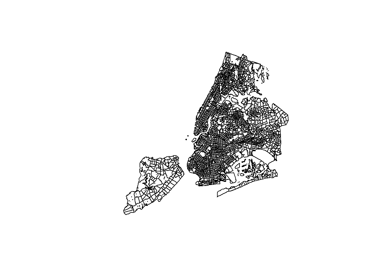

Next we clean up the 311 data and convert the state plane coordinates from the 311 data into an sf object using the st_as_sf function.

# create points by x, y 
points <- hh311_new %>%
  na.omit() %>% 
  arrange(op_date) %>% 
  mutate(svc_qty = as.numeric(svc_qty),
         # calls at same exact time combined to 1 
         svc_qty = ifelse(svc_qty > 1, 1, svc_qty)) %>% 
  filter(resp_hr > 0,        # drops 9 records
         resp_hr < 15*24,    # drops 679 records greater than 15 days
         op_date > date("2017-10-1")
         ) %>% 
  mutate(op_dow = weekdays.Date(op_date), 
         cl_dow = weekdays.Date(cl_date), 
         borough = gsub("(?<=\\b)([a-z])", "\\U\\1", 
                        tolower(borough), perl=TRUE)) %>% 
  st_as_sf(coords = c("x_sp", "y_sp"), 
           crs = 2263,       # EPSG for NY/LI to match census data
           remove = T)       # Drop the original x/y columns

points %>% glimpse(width = 60)

## Rows: 213,043
## Columns: 13
## $ borough        <chr> "Brooklyn", "Manhattan", "Manhattan~
## $ city           <chr> "BROOKLYN", "NEW YORK", "NEW YORK",~
## $ agency         <chr> "HPD", "HPD", "HPD", "HPD", "HPD", ~
## $ complaint_type <chr> "HEAT/HOT WATER", "HEAT/HOT WATER",~
## $ incident_zip   <chr> "11221", "10031", "10023", "11235",~
## $ address        <chr> "591 MADISON STREET", "515 WEST  14~
## $ svc_qty        <dbl> 1, 1, 1, 1, 1, 1, 1, 1, 1, 1, 1, 1,~
## $ op_date        <dttm> 2017-10-01 00:06:02, 2017-10-01 00~
## $ cl_date        <dttm> 2017-10-04 10:34:31, 2017-10-05 02~
## $ resp_hr        <dbl> 82.47472, 97.99611, 102.00194, 72.6~
## $ op_dow         <chr> "Sunday", "Sunday", "Sunday", "Sund~
## $ cl_dow         <chr> "Wednesday", "Thursday", "Thursday"~
## $ geometry       <POINT [US_survey_foot]> POINT (1002578 1~

Now we use the geometry from the census data (nyc) to obtain the census block codes for each record from the 311 data via st_join. I do this to then aggregate by census block ID to obtain the counts of service requests and the average open-to-close duration for each census block.

ct_check <- st_join(points, nyc[, "ct"], join = st_within) %>% as_tibble()

z<-as_tibble(nyc) %>% 
  left_join(as_tibble(ct_check), by = "ct")  %>% as.data.frame() %>% 
  mutate(svc_qty = ifelse(is.na(svc_qty) & !is.na(ct_med_inc), 0, svc_qty))

# z %>% filter(is.na(ct_med_inc))

# z %>% filter(svc_qty==0) %>%
#   arrange(desc(ct_med_inc))
# z %>% filter(svc_qty==0) %>% ggplot(aes(x = ct_med_inc))+geom_histogram()

# z %>% 
#   mutate(svc_qty = ifelse(is.na(svc_qty) & !is.na(ct_med_inc), 1, svc_qty)) %>% 
#   filter(is.na(ct_med_inc))
# # z %>% group_by(ct, 
#                ct_med_inc, ct_gini) %>% 
#   summarise(qty = sum(svc_qty)) %>% 
#   ungroup() %>% 
#   summarise(sum(qty, na.rm = T))

# getting all the ct codes for points
# summarise by ct block-level
ct_311 <- st_join(points, nyc[, "ct"], join = st_within) %>% 
  as_tibble() %>% 
  group_by(ct, borough) %>% 
  summarise(svc_qty = sum(svc_qty), 
            sr_dur = mean(resp_hr))

## `summarise()` has grouped output by 'ct'. You can override using the `.groups` argument.

map_data <- nyc %>%
  left_join(as_tibble(ct_311), by = "ct") %>% 
  mutate(qty_per_1k = svc_qty*1000/ct_pop_renters) %>% 
  filter(!is.infinite(qty_per_1k))

map_data %>% glimpse(width = 60)

## Rows: 2,148
## Columns: 9
## $ ct             <chr> "36005000200", "36005000400", "3600~
## $ ct_med_inc     <dbl> 70893, 76667, 31540, 39130, 17083, ~
## $ ct_gini        <dbl> 0.4021, 0.3636, 0.4343, 0.4626, 0.5~
## $ ct_pop_renters <dbl> 2175, 1593, 4794, 1938, 7340, 4796,~
## $ borough        <chr> "Bronx", "Bronx", "Bronx", "Bronx",~
## $ svc_qty        <dbl> 38, 35, 139, 142, 141, 1, 5, 219, 4~
## $ sr_dur         <dbl> 124.62179, 91.33221, 93.50885, 99.5~
## $ geometry       <GEOMETRY [US_survey_foot]> POLYGON ((102~
## $ qty_per_1k     <dbl> 17.4712644, 21.9711237, 28.9945766,~

And below we plot our choropleth map. Be sure to check out the getting started vignette for tmap map options and run the tmaptools::palette_explorer() to experiment with different color palettes.

tmap_mode("plot")
tm1 <- tm_shape(map_data) +
  tm_polygons("qty_per_1k", 
              style = "quantile",
              legend.hist = F, 
              palette = "Reds",
              n = 7, 
              border.alpha = .2, 
              showNA = T, 
              title = "Heat/Hot Water Calls\nper 1K Renter Pop.", 
              legend.hist.z = 300)

tm2 <- tm_shape(map_data) +
  tm_polygons("sr_dur", 
              trans = "log10",
              style = "quantile",
              legend.hist = T, 
              palette = "RdBu",
              contrast = c(0, 1),
              n = 7, 
              border.alpha = .2, 
              showNA = T, 
              title = "SR Open-to-Close Hours\n311 Heat/Hot Water")

tmap_arrange(tm1, tm2, ncol = 1)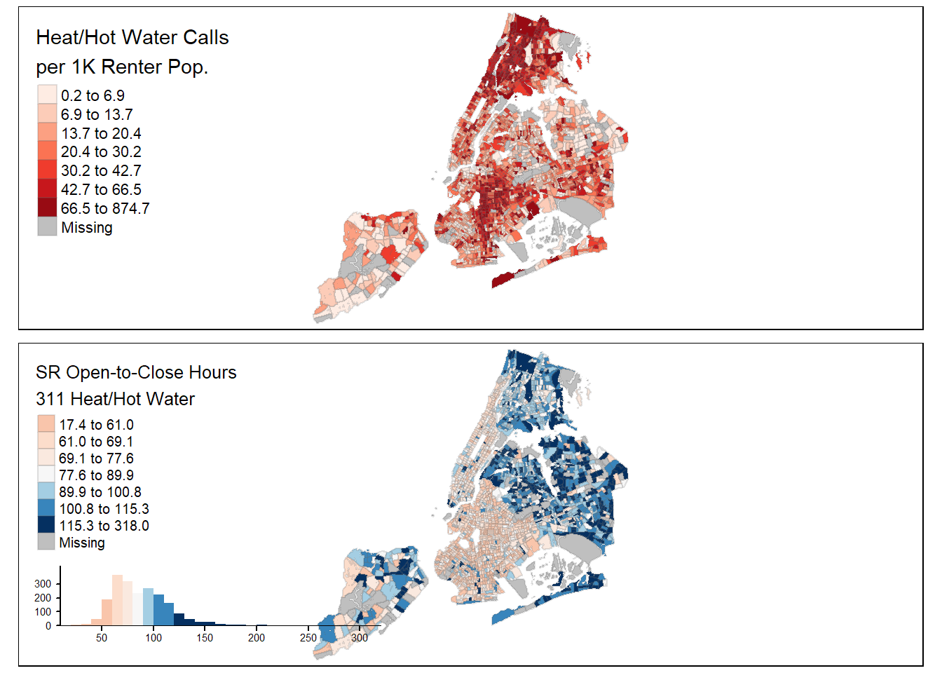

Interactive, java-script maps are also possible with tmap! While the below map isn’t interactive - it’s just a screen-cap of the actual map - it’s nice to know the option is available. I decided not to embed it here as the performance was too sluggish on my blog’s no-cost hosting service.

# Code for the above, leaflet/tmap version of the plots:
dollar_format <- function(x) {
  paste0("$", formatC(x/1000, digits = 1, format = "f"), "K")
}

tmap_mode("view")
my_map <- tm_shape(map_data) +
  tm_polygons(c("qty_per_1k","sr_dur"),
              border.alpha = .05,
              legend.text.size=.5,
              style="quantile",
              palette = list("Reds", "RdBu"),
              n = c(7, 9),
              title = c("SRs Per1K Renters",
                        "Response Duration Hours"),
              popup.vars = c("Borough"= "borough",
                             "SRs/1K Renters" = "qty_per_1k",
                             "Median Income"= "ct_med_inc"),
              popup.format = list(qty_per_1k=list(digits=2),
                                  ct_med_inc=list(fun = dollar_format)))+
  tm_view(alpha = 1, text.size.variable = TRUE,
          view.legend.position = c("left", "bottom"),
          set.zoom.limits = c(10,13))+
  tm_facets(sync = T, ncol = 2)

tmap_leaflet(my_map)

That concludes today’s post! There’s a ton to learn about map data and I’ve included some helpful references below to get you started.