Predicting Car Crashes with Insurance Data
Purpose
Today I review a data set containing information on approximately 8,000 customers of an insurance company. Each record contains two response variables that indicate whether a customer was in a car crash or not and how much said car-crash cost.
library(tidyverse)
library(stargazer)
library(GGally)
library(kableExtra)
library(ResourceSelection)
library(RCurl)
library(pROC)
clr_dollar <- function(x){
# cleans out commas and $ of string-formatted currency
return(as.numeric(gsub('[$,]','',x)))
}
# Mappings to clean-up data entries for easier manipulation and analysis
job_map <- data.frame(JOB = c("Doctor", "Lawyer", "Professional",
"Manager", "z_Blue Collar", "Clerical",
"Home Maker", "Student", ""),
EMPL = c("Doc", "Law", "Pro", "Mgr", "BC",
"Cler", "HM", "Stu", "-")) # '-' instead of blank
urb_map <- data.frame(URBANICITY = c("Highly Urban/ Urban",
"z_Highly Rural/ Rural"),
URBCITY = c("Urb", "Rur"))
edu_map <- data.frame(EDUCATION = c("<High School", "z_High School",
"Bachelors", "Masters", "PhD"),
EDU = c("HS", "HS", "BS", "MS", "PhD"))
car_map <- data.frame(CAR_TYPE = c("Minivan", "z_SUV", "Sports Car",
"Van", "Panel Truck", "Pickup"),
CTYPE = c("MV", "SUV", "Sprt", "Van",
"panTr", "pikTr"))
carU_map <- data.frame(CAR_USE = c("Commercial", "Private"),
CAR_U = c("Comm", "Priv"))
my_theme <- function(){
theme(panel.background = element_rect(fill = 'grey92', color = NA),
panel.grid = element_line(color = 'white'),
strip.background = element_rect(fill = "grey85", colour = NA),
plot.margin = margin(.1, .1, .1, .1, "cm"),
legend.position="none",
strip.text = element_text(color = "black", face = "bold", size = rel(.8)),
axis.title.x=element_blank(),
axis.title.y=element_blank())
}Data Pre-Processing
Several actions were taken ensure the data was ready for analysis:
- Cleaned up consistency of factors (e.g.
z_Fchanged tofunderSEX) - Shortened string names of factors for categorical variables (e.g.
ProfessionaltoPro) - Added
tagfield to identify the sets ofTARGET_FLAG(e.g.1 = crashvs.0 = safe) - Stripped out any non-standard characters from numerical entries (e.g.
$and,)
# Repair data types, normalize factors, shorten entries, re-order columns
read_ins_factor <- function(filename){
  insur <- read_csv(filename) %>%
  mutate(INCOME = clr_dollar(INCOME),
         HOME_VAL = clr_dollar(HOME_VAL),
         BLUEBOOK = clr_dollar(BLUEBOOK),
         OLDCLAIM = clr_dollar(OLDCLAIM),
         REVOKED = as.factor(tolower(REVOKED)),
         PARENT1 = as.factor(tolower(PARENT1)),
         MSTATUS = as.factor(ifelse(MSTATUS=='z_No', 'no', 'yes')),
         SEX = as.factor(ifelse(SEX == 'z_F', 'f', 'm')),
         RED_CAR = as.factor(RED_CAR),
         tag = ifelse(TARGET_FLAG == 1, 'crash', 'safe')) %>%
    left_join(job_map, by = "JOB") %>%
    left_join(urb_map, by = "URBANICITY") %>%
    left_join(edu_map, by = "EDUCATION") %>%
    left_join(car_map, by = "CAR_TYPE") %>%
    left_join(carU_map, by = "CAR_USE") %>%
  select_('tag', 'TARGET_FLAG', 'TARGET_AMT', 'KIDSDRIV', 'AGE',
       'HOMEKIDS', 'YOJ', 'TRAVTIME', 'TIF', 'CLM_FREQ',
       'MVR_PTS', 'CAR_AGE', 'INCOME', 'HOME_VAL',
       'BLUEBOOK', 'OLDCLAIM', 'PARENT1', 'MSTATUS',
       'SEX','RED_CAR', 'REVOKED','URBCITY', 'CAR_U',
       'EDU', 'CTYPE', 'EMPL') %>%
  rename(JOB = EMPL, URBANICITY = URBCITY, EDUCATION = EDU,
         CAR_TYPE = CTYPE, CAR_USE = CAR_U)
}

ins_url <- paste0("https://raw.githubusercontent.com/jbrnbrg/",
                  "msda-datasets/master/insurance_training_data.csv")
ins_ev_url <- paste0("https://raw.githubusercontent.com/jbrnbrg/",
                     "msda-datasets/master/insurance-evaluation-data.csv")

insurf <- read_ins_factor(ins_url)

stat_info = describe(insurf) %>%
  as.data.frame()
Data Exploration
Summary findings:
- 8161 total records with 25 variables: 2 response, 13 numerical, 7 binary, 3 categorical
- Many
NAs:CAR_AGE: 510,HOME_VAL: 464,YOJ: 454,INCOME: 445,AGE: 6 - Collinearity present in at least one variable pair
Data preview:
A preview of 4 random records of insurance_training_data.csv used to develop the model. As there are 26 variables, the preview is broken into 3 parts:
| TARGET_FLAG | TARGET_AMT | KIDSDRIV | AGE | HOMEKIDS | YOJ | TRAVTIME | TIF | CLM_FREQ | MVR_PTS |
|---|---|---|---|---|---|---|---|---|---|
| 0 | 0 | 0 | 46 | 0 | 11 | 13 | 1 | 3 | 6 |
| 0 | 0 | 2 | 45 | 3 | 14 | 28 | 11 | 0 | 3 |
| 0 | 0 | 0 | 42 | 0 | NA | 36 | 8 | 0 | 1 |
| 1 | 4085 | 0 | 28 | 1 | 9 | 32 | 7 | 3 | 6 |
knitr::kable(head(t2, n=4), format = 'markdown', booktabs = T) %>%
  row_spec(0, bold = T) %>%
kable_styling(font_size = 5, position = "left", full_width = F)| CAR_AGE | INCOME | HOME_VAL | BLUEBOOK | OLDCLAIM | PARENT1 | MSTATUS | SEX | RED_CAR | REVOKED |
|---|---|---|---|---|---|---|---|---|---|
| 15 | 104017 | 0 | 21610 | 28005 | no | no | m | no | no |
| 10 | 60769 | 218782 | 8310 | 0 | no | yes | m | no | no |
| 15 | 107562 | 281386 | 21600 | 0 | no | yes | f | no | no |
| 1 | NA | 0 | 24560 | 20778 | yes | no | f | no | yes |
knitr::kable(head(t3, n=4), format = 'markdown', booktabs = T) %>%
  row_spec(0, bold = T) %>%
kable_styling(font_size = 5, position = "left", full_width = F)| URBANICITY | CAR_USE | EDUCATION | CAR_TYPE | JOB |
|---|---|---|---|---|
| Urb | Comm | MS | Van | NA |
| Urb | Priv | BS | MV | Mgr |
| Urb | Priv | BS | SUV | Mgr |
| Urb | Comm | HS | SUV | BC |
Summary statistics:
The below table provides the summary statistics. Variables with an * are binary/categorical variables.| n | mean | sd | median | min | max | skew | kurtosis | se | |
|---|---|---|---|---|---|---|---|---|---|
| TARGET_FLAG | 8161 | 0 | 0 | 0 | 0 | 1 | 1 | -1 | 0 |
| TARGET_AMT | 8161 | 1504 | 4704 | 0 | 0 | 107586 | 9 | 112 | 52 |
| KIDSDRIV | 8161 | 0 | 1 | 0 | 0 | 4 | 3 | 12 | 0 |
| AGE | 8155 | 45 | 9 | 45 | 16 | 81 | 0 | 0 | 0 |
| HOMEKIDS | 8161 | 1 | 1 | 0 | 0 | 5 | 1 | 1 | 0 |
| YOJ | 7707 | 10 | 4 | 11 | 0 | 23 | -1 | 1 | 0 |
| TRAVTIME | 8161 | 33 | 16 | 33 | 5 | 142 | 0 | 1 | 0 |
| TIF | 8161 | 5 | 4 | 4 | 1 | 25 | 1 | 0 | 0 |
| CLM_FREQ | 8161 | 1 | 1 | 0 | 0 | 5 | 1 | 0 | 0 |
| MVR_PTS | 8161 | 2 | 2 | 1 | 0 | 13 | 1 | 1 | 0 |
| CAR_AGE | 7651 | 8 | 6 | 8 | -3 | 28 | 0 | -1 | 0 |
| INCOME | 7716 | 61898 | 47573 | 54028 | 0 | 367030 | 1 | 2 | 542 |
| HOME_VAL | 7697 | 154867 | 129124 | 161160 | 0 | 885282 | 0 | 0 | 1472 |
| BLUEBOOK | 8161 | 15710 | 8420 | 14440 | 1500 | 69740 | 1 | 1 | 93 |
| OLDCLAIM | 8161 | 4037 | 8777 | 0 | 0 | 57037 | 3 | 10 | 97 |
| PARENT1* | 8161 | 1 | 0 | 1 | 1 | 2 | 2 | 3 | 0 |
| MSTATUS* | 8161 | 2 | 0 | 2 | 1 | 2 | 0 | -2 | 0 |
| SEX* | 8161 | 1 | 0 | 1 | 1 | 2 | 0 | -2 | 0 |
| RED_CAR* | 8161 | 1 | 0 | 1 | 1 | 2 | 1 | -1 | 0 |
| REVOKED* | 8161 | 1 | 0 | 1 | 1 | 2 | 2 | 3 | 0 |
| URBANICITY* | 8161 | 2 | 0 | 2 | 1 | 2 | -1 | 0 | 0 |
| CAR_USE* | 8161 | 2 | 0 | 2 | 1 | 2 | -1 | -2 | 0 |
| EDUCATION* | 8161 | 2 | 1 | 2 | 1 | 4 | 1 | -1 | 0 |
| CAR_TYPE* | 8161 | 3 | 2 | 3 | 1 | 6 | 0 | -1 | 0 |
| JOB* | 7635 | 4 | 3 | 4 | 1 | 8 | 0 | -2 | 0 |
Continuous Variables:
The below plots employ binomial smoothing to highlight the probability of a crash over the range of variable values.
binomial_smooth <- function(...){
  # Via: http://ggplot2.tidyverse.org/reference/geom_smooth.html
  geom_smooth(method='glm',  method.args = list(family = 'binomial'), ...)
}

insurf %>% select(-c(17:26)) %>%
  gather(-c(TARGET_AMT, TARGET_FLAG, tag), key = "var", value = "val") %>%
  ggplot(aes(x = val, y = TARGET_FLAG)) +
  geom_point(aes(color=tag),
             position=position_jitter(height=.3, width=0),
             alpha=.05) +
  binomial_smooth(formula = y ~ splines::ns(x, 2)) +
  facet_wrap(~ var, ncol =5, scales = "free_x") + my_theme()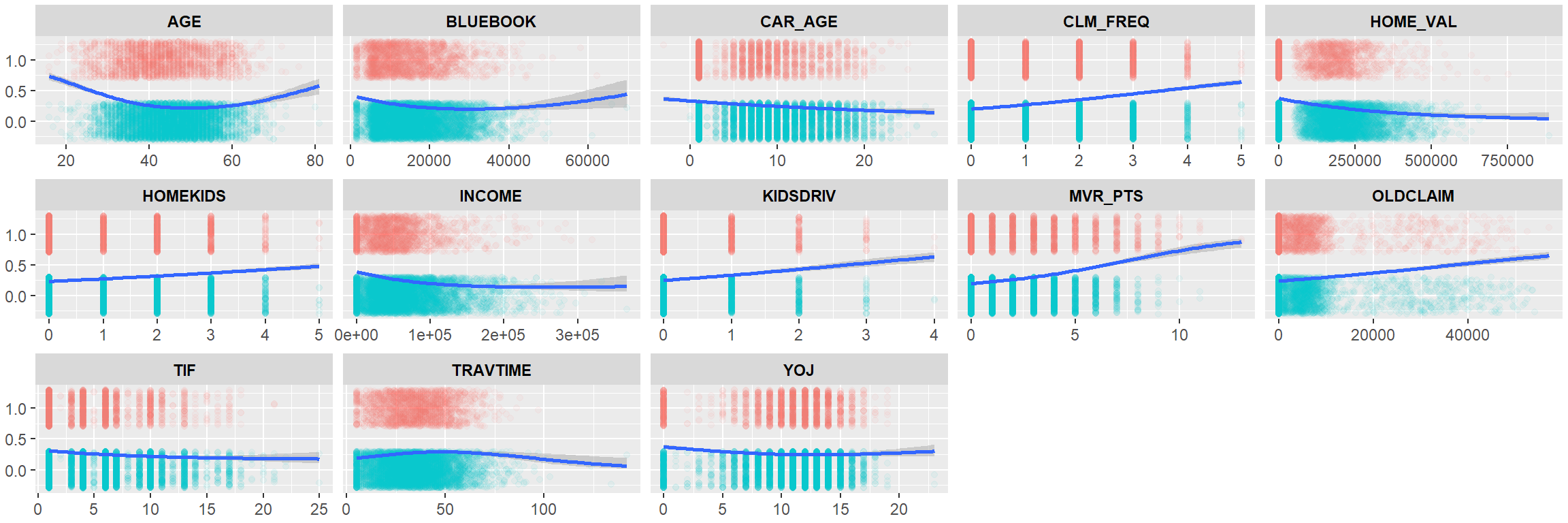
# imputed %>% select(-c(17:26)) %>%
#   gather(-c(TARGET_AMT, TARGET_FLAG, tag), key = "var", value = "val") %>%
#   ggplot(aes(x = val, y = TARGET_FLAG)) +
#   geom_point(aes(color=tag),
#              position=position_jitter(height=.3, width=0),
#              alpha=.05) +
#   binomial_smooth(formula = y ~ splines::ns(x, 2)) +
#   facet_wrap(~ var, ncol =5, scales = "free_x") + my_theme()
The primary take-aways from the above visualization:
- As
CAR_AGE,HOME_VALUE,INCOMEorTIFincreases, the probability of a crash decreases. MVR_PTSappears to be a good predictor of crashes.- The remaining points appear to have some polynomial relationship - i.e. there’s some point between low and high variable values that represents a maxima or minima of crash probability before changing direction.
Further, the below visualization provides histograms for each of the continuous variables on log scales for y separated by the crash/safe tag. These plots support the above take-aways for the continuous variables:
insurf %>% select(-c(17:26)) %>%
  gather(-c(TARGET_AMT, TARGET_FLAG, tag), key = "var", value = "val") %>%
  ggplot(aes(x = val, fill = tag, color = tag)) +
  geom_histogram(alpha=.4) + scale_y_log10() +
  facet_wrap(~ var, ncol =5, scales = "free_x") + my_theme()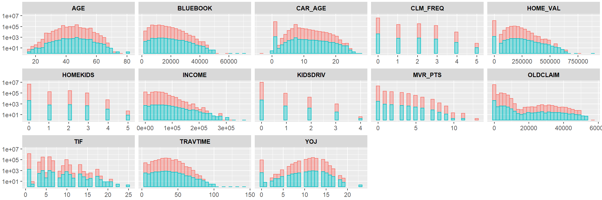
The above plot highlights the splits between crash/safe among the continuous variables. Note that as TRAVTIME, INCOME, HOMEKIDS, KIDDRIV, MVR_PTS, and TIF increases, the presence of crashes decreases.
Categorical Variables:
The below visualization provides a way to review the density of the crash/safe populations among the categorical variables in the data:
# binary and categorical
insurf %>%
select(names(insurf)[c(1:3,17:26)]) %>% ungroup() %>%
gather(-c(tag, TARGET_FLAG, TARGET_AMT), key = "var", value = "val") %>%
ggplot(aes(x = val, y=tag, color = tag)) +
geom_jitter(alpha = .1) + #scale_y_log10(labels = scales::comma) +
facet_wrap(~ var, scales = "free_x", ncol =5) + my_theme()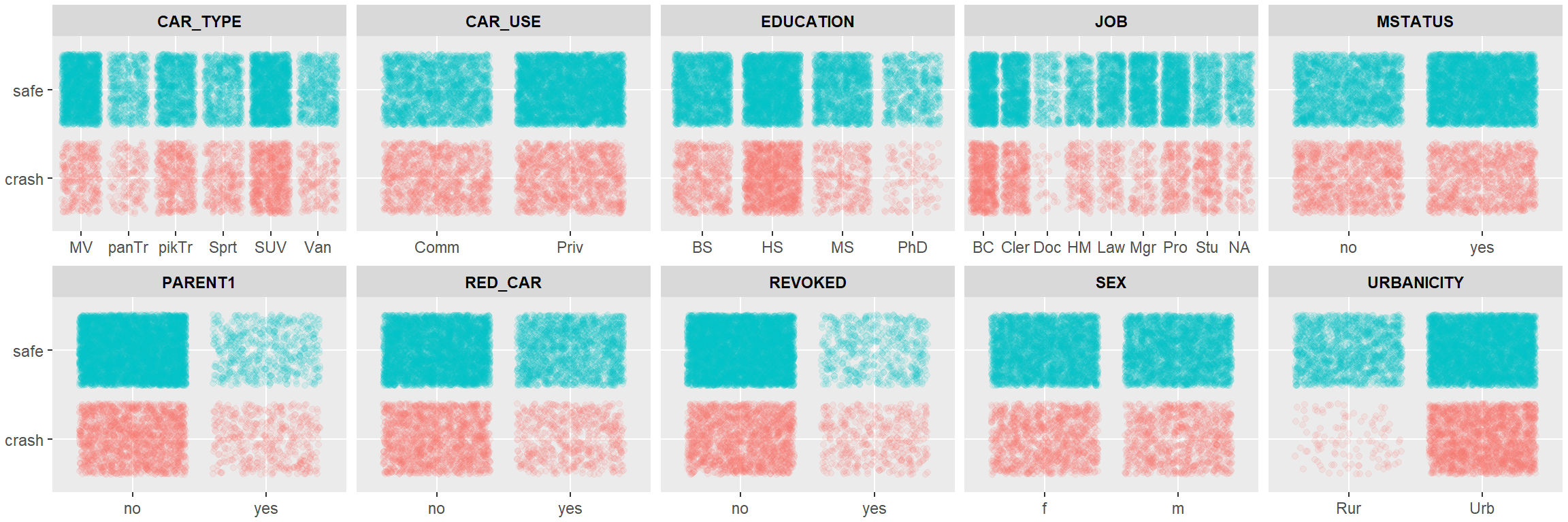 The summary findings from the above visualization are with respect to an apparent higher presence of crashes:
CAR_TYPE= SUVEDUCATION= High School (HS)JOB= Blue Collar (BC)PARENT1= non-single parent households (no)URBANCITY= Urban (Urb)
Each of these could be population specific, however. Next, I’ve provided violin plots for the TARGET_AMT for each of the continuous variables strictly among those who have crashed. The width of the violins is proportional to the sample size:
# binary and categorical
insurf %>% filter(TARGET_FLAG != 0) %>%
  select(names(insurf)[c(1:3,17:26)]) %>% ungroup() %>%
  gather(-c(tag, TARGET_FLAG, TARGET_AMT), key = "var", value = "val") %>%
  ggplot(aes(x = val, y=TARGET_AMT, fill = var)) +
  geom_violin(alpha = .5,
              draw_quantiles = c(0.25, 0.5, 0.75),
              adjust = .8, scale = "count") +
  scale_y_log10(labels = scales::comma) +
  facet_wrap(~ var, scales = "free_y", ncol =5) + coord_flip() + my_theme()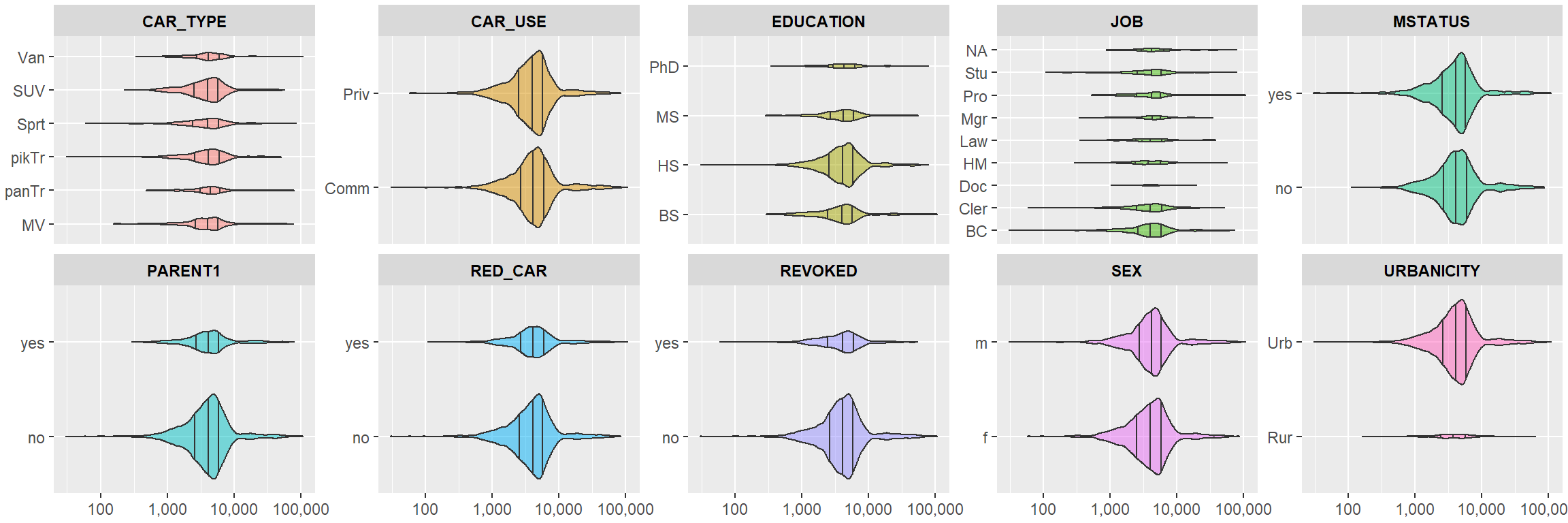
Model Build
First I will create and select a logit regression to be able to predict whether a crash is likely and then create and select a linear regression to predict crash cost.
Logistic
I created 3 glm models m1, m2, and m3 and selected them based on the AIC score. I performed additional review comparing the results of their Hosmer-lemeshow fit tests for the binary response TARGET_FLAG that I’ve included in the code.
insur.no.na <- insurf %>% na.omit()

# Model 1: All variables included ******************************
m1 <- glm(TARGET_FLAG ~  KIDSDRIV + AGE + HOMEKIDS + YOJ + TRAVTIME +
            TIF + CLM_FREQ + MVR_PTS + CAR_AGE + INCOME + HOME_VAL +
            BLUEBOOK + OLDCLAIM + PARENT1 + MSTATUS + SEX + RED_CAR +
            REVOKED + URBANICITY + CAR_USE + EDUCATION + CAR_TYPE +
            JOB, data = insur.no.na, family = "binomial")

# Model 2: uses variables from: car::Anova(MASS:stepAIC(m1)) ***
m2 <- glm(TARGET_FLAG ~  KIDSDRIV + TRAVTIME + TIF + CLM_FREQ + MVR_PTS +
            INCOME + HOME_VAL + BLUEBOOK + OLDCLAIM + PARENT1 + MSTATUS +
            REVOKED + URBANICITY + CAR_USE + EDUCATION + CAR_TYPE + JOB,
          data = insur.no.na, family = "binomial")

# Model 3: is m2 w/out HOME_VAL ********************************
m3 <- glm(TARGET_FLAG ~  KIDSDRIV + TRAVTIME + TIF + CLM_FREQ + MVR_PTS +
            INCOME + BLUEBOOK + OLDCLAIM + PARENT1 + MSTATUS +
            REVOKED + URBANICITY + CAR_USE + EDUCATION + CAR_TYPE + JOB,
          data = insur.no.na, family = "binomial")
# hoslem.test(insur.no.na$TARGET_FLAG, fitted(m1))
# hoslem.test(insur.no.na$TARGET_FLAG, fitted(m2))
# hoslem.test(insur.no.na$TARGET_FLAG, fitted(m3))
Logistic Eval/Selection:
The summaries of each of the models created are shown below:
stargazer(m1, m2, m3,
          type = 'latex',
          column.sep.width = "1pt",
          single.row = T,
          omit.stat = c('ser'),
          header = F)
As shown above, M2 has the lowest AIC. Below, I have completed the diagnostics on each of the models - the ROC curves and table entries below are in the order of the models:
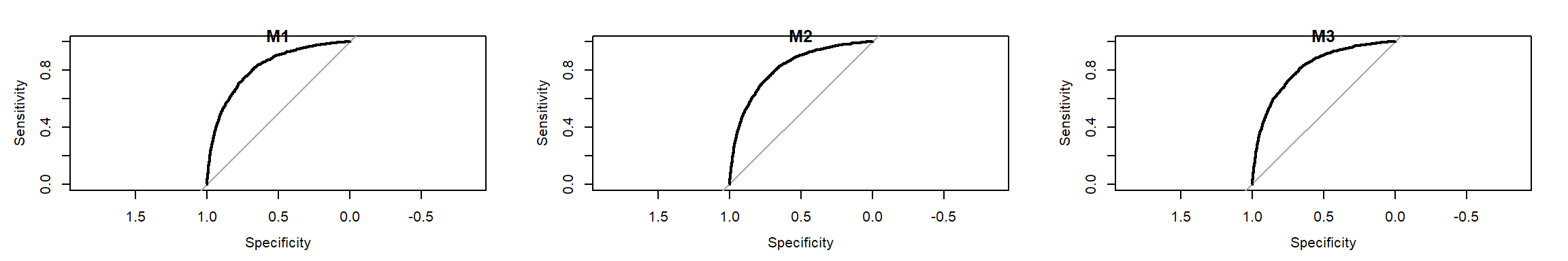
As shown above, there is little difference between the plots.
| AIC | accuracy | class_err | precise | sensitive | specific | f1_score | AUC |
|---|---|---|---|---|---|---|---|
| 5434.272 | 0.7932175 | 0.2067825 | 0.6682600 | 0.4363296 | 0.9218996 | 0.5279456 | 0.8186477 |
| 5429.962 | 0.7943755 | 0.2056245 | 0.6711153 | 0.4394507 | 0.9223498 | 0.5311203 | 0.8179944 |
| 5439.371 | 0.7932175 | 0.2067825 | 0.6702128 | 0.4325843 | 0.9232501 | 0.5257967 | 0.8170804 |
I note that there’s little difference between the 3 sets of scores. I choose m2 because it has the lowest AIC, and slightly fewer variables than the original set:
## glm(formula = TARGET_FLAG ~ KIDSDRIV + TRAVTIME + TIF + CLM_FREQ +
##     MVR_PTS + INCOME + HOME_VAL + BLUEBOOK + OLDCLAIM + PARENT1 +
##     MSTATUS + REVOKED + URBANICITY + CAR_USE + EDUCATION + CAR_TYPE +
##     JOB, family = "binomial", data = insur.no.na)
Linear Model:
I created 3 lm models linM1, linM2, and linM3 and selected them based on the R^2 and residual analysis. Each linear model was refined using MASS::stepAIC.
Linear Eval/Selection
After several iterations and reviews I settled on the second linear model linM2_step. While the R^2 was the best, I use this model with some reservation given the results of the below residual analysis - these do not appear normal.
# col_labels = c("model1", "model2", "model3")
# coefs = c(m1$coefficients, m2$coefficients, m3$coefficients)
stargazer(linM1_step, linM2_step, linM3_step,
          type = 'html',
          column.sep.width = "1pt",
          single.row = T,
          omit.stat = c('ser'),
header = F)| Dependent variable: | |||
| TARGET_AMT | log(TARGET_AMT + 1) | (TARGET_AMT + 1) | |
| (1) | (2) | (3) | |
| KIDSDRIV | 217.739* (113.522) | 0.386*** (0.083) | -0.048*** (0.010) |
| TRAVTIME | 11.061*** (3.608) | 0.018*** (0.003) | -0.002*** (0.0003) |
| TIF | -44.805*** (13.673) | -0.063*** (0.010) | 0.007*** (0.001) |
| CLM_FREQ | 0.264*** (0.045) | -0.033*** (0.005) | |
| MVR_PTS | 184.040*** (27.039) | 0.189*** (0.021) | -0.022*** (0.003) |
| CAR_AGE | -27.544* (14.399) | ||
| INCOME | -0.00000** (0.00000) | 0.00000*** (0.00000) | |
| HOME_VAL | -0.002** (0.001) | -0.00000*** (0.00000) | |
| BLUEBOOK | -0.00002*** (0.00001) | 0.00000*** (0.00000) | |
| OLDCLAIM | -0.00002*** (0.00001) | 0.00000*** (0.00000) | |
| PARENT1yes | 528.163*** (195.907) | 0.763*** (0.144) | -0.088*** (0.017) |
| MSTATUSyes | -478.386*** (154.050) | -0.500*** (0.117) | 0.079*** (0.012) |
| SEXm | 302.750* (161.942) | 0.251* (0.148) | |
| RED_CARyes | -0.268** (0.125) | ||
| REVOKEDyes | 443.978** (173.335) | 1.175*** (0.143) | -0.143*** (0.017) |
| URBANICITYUrb | 1,678.558*** (149.773) | 2.439*** (0.113) | -0.290*** (0.013) |
| CAR_USEPriv | -693.703*** (174.442) | -1.079*** (0.128) | 0.128*** (0.015) |
| EDUCATIONHS | 215.761 (168.255) | 0.544*** (0.115) | -0.064*** (0.014) |
| EDUCATIONMS | 50.920 (249.731) | 0.015 (0.176) | -0.001 (0.021) |
| EDUCATIONPhD | 730.822** (346.171) | 0.588** (0.255) | -0.066** (0.030) |
| CAR_TYPEpanTr | 691.566** (297.048) | 0.645*** (0.239) | -0.079*** (0.027) |
| CAR_TYPEpikTr | 415.945** (185.211) | 0.591*** (0.137) | -0.069*** (0.016) |
| CAR_TYPESprt | 1,195.211*** (221.704) | 1.288*** (0.172) | -0.145*** (0.017) |
| CAR_TYPESUV | 850.150*** (179.344) | 0.933*** (0.142) | -0.103*** (0.013) |
| CAR_TYPEVan | 566.810** (234.540) | 0.559*** (0.177) | -0.068*** (0.020) |
| JOBCler | -139.469 (206.070) | 0.236 (0.153) | -0.031* (0.018) |
| JOBDoc | -1,453.438*** (492.990) | -1.038*** (0.363) | 0.119*** (0.043) |
| JOBHM | -199.516 (269.640) | -0.067 (0.209) | 0.007 (0.024) |
| JOBLaw | -315.007 (335.933) | -0.206 (0.247) | 0.024 (0.029) |
| JOBMgr | -1,210.374*** (250.123) | -1.187*** (0.184) | 0.139*** (0.022) |
| JOBPro | -105.704 (228.042) | -0.161 (0.168) | 0.023 (0.020) |
| JOBStu | -372.302 (243.145) | -0.070 (0.184) | -0.006 (0.021) |
| Constant | 227.456 (342.076) | 0.272 (0.284) | 0.956*** (0.029) |
| Observations | 6,045 | 6,045 | 6,045 |
| R2 | 0.075 | 0.235 | 0.235 |
| Adjusted R2 | 0.071 | 0.231 | 0.232 |
| F Statistic | 18.165*** (df = 27; 6017) | 59.570*** (df = 31; 6013) | 66.153*** (df = 28; 6016) |
| Note: | p<0.1; p<0.05; p<0.01 | ||
The below plots suggest that my linear model has some underlying relationships that haven’t been addressed but the prediction power remains. Further training and transformation will result in improved results.
par(mfrow=c(1,2))
plot(linM2_step,which=c(2,2))
hist(linM2_step$residuals)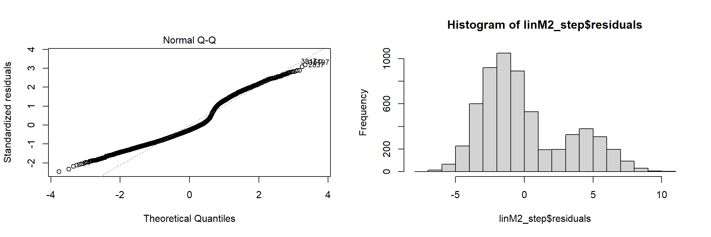
par(mfrow=c(1,1))