Binary Response and GGally
If I am working on data with a binary response, I like to use the GGally package for its ggpairs function. It provides a way to look at a lot of different data types at the same time but the setup and customization can be a little daunting. In this example, which leverages this crime data, I demonstrate how ggpairs can be used to reveal a lot of information in a single figure.
crimes <- read.csv("crime-training-data.csv", header = T) %>%# read in data
  mutate(tag=ifelse(target==1, 'a', 'b'),                    # tag for colors
         chas=ifelse(chas==1, 'bo','no')) %>% select(-black)

cr_exp <- crimes %>%
  select(-tag) %>% mutate(chas=ifelse(chas=='brdrs', 1, 0))  # crimes, no tag

stat_info = psych::describe(cr_exp) %>%
  as.data.frame()

pm <- ggpairs(crimes, columns = c('rm','medv','lstat', 'dis',
                                  'age','nox', 'indus', 'tax',
                                  'ptratio', 'rad', 'zn', 'chas'),
 mapping = ggplot2::aes(color = tag),
 lower = list(continuous = wrap('points', size = 1, alpha = .4),
              combo = 'facetdensity'),
 upper = list(continuous =  wrap("cor", size = 3, alpha = 1),
              combo = 'box_no_facet'),
 diag = list(continuous = wrap('densityDiag', alpha = .6))) +
  theme(panel.background = element_rect(fill = 'grey92', color = NA),
        panel.spacing = unit(1, "pt"),
        panel.grid = element_line(color = 'white'),
        strip.background = element_rect(fill = "grey85", colour = NA),
        plot.margin = margin(.1, .1, .1, .1, "cm"))
pm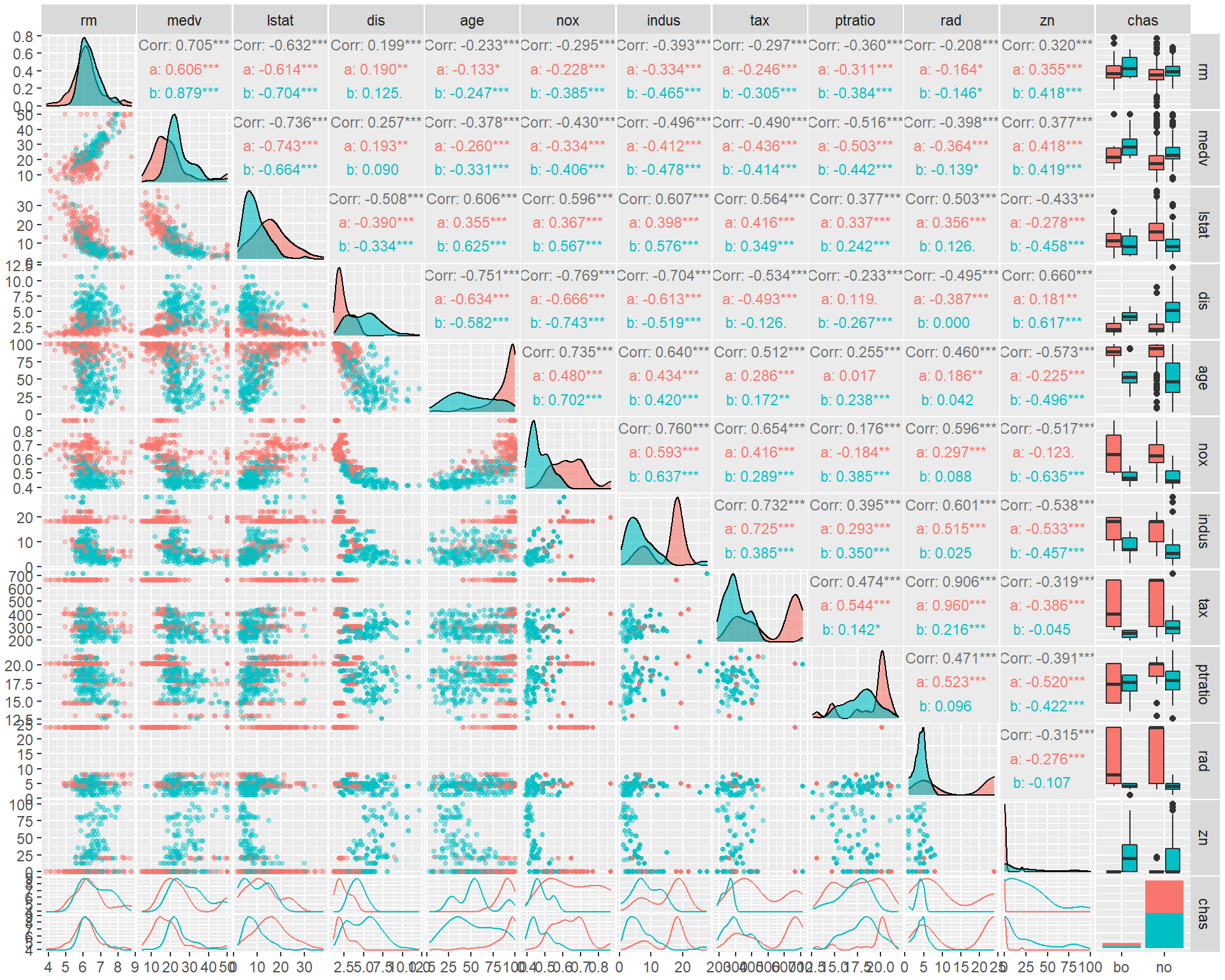
2019-01-13