Predicting House Sale Price with the Ames Housing Data
In this post I’m going to perform simplified bottoms-up EDA, model development, prediction, and model evaluation using a public data set that contains data for houses that sold in Ames, Iowa. This post essentially revisits a previous analysis I performed in a group for my MS degree program at CUNY. The main differences here will be that my analysis will be abbreviated to illustrate my skillset, I’ll be using python instead of R, and I will be relying on python’s fantastic scikit-learn library to perform the regressions.
You can find out more about scikit-learn, better known as sklearn, here.
Data Background
Each of over 2,900 observations in the data represent attributes of an individual residential properties sold in Ames, Iowa between 2006 through 2010. There are 79 variables included that cover a multitude of property attributes including physical appearance, measures of quality and condition, and various continuous measures such as square footage. The data types are varied and include discrete, continuous, and categorical (both nominal and ordinal) data. I will be leveraging these features to predict the target variable of SalePrice.
The data was originally published in the Journal of Statistics Education (Volume 19, Number 3) but the data I am using in this post originally came from this kaggle competition. Note that only the amestrain.csv data contains the target variable for this exercise.
Python Libraries
import pandas as pd                                         # Data Wrangle
import numpy as np
%matplotlib inline

import matplotlib.pyplot as plt                             # Visuals & EDA
import seaborn as sns

from scipy.stats import skew                                # Transformation
from scipy.special import boxcox1p

from sklearn.preprocessing import LabelEncoder, RobustScaler# Pre-processing
from sklearn.pipeline import make_pipeline

from sklearn.linear_model import Lasso, ElasticNet          # Modeling
from sklearn.ensemble import GradientBoostingRegressor

from sklearn.model_selection import cross_val_score         # Evaluation
from sklearn.model_selection import KFold
from sklearn.metrics import mean_squared_error, mean_absolute_error

import warnings
warnings.filterwarnings(action="ignore", message="^internal gelsd")

plt.rcParams['figure.figsize'] = [12, 4]
EDA
Although this data contains both training and testing sets (amestrain.csv & amestest.csv, respectively), the kaggle competition data doesn’t contain the actual sale prices for the test set so my model building and evaluation will be limited to to the training set. However, I will proceed with the data exploration and preperation as if the data were complete.
Let’s get started by downloading the data and taking look at the shape and dtypes:
# Ames Housing Files
b_url = "https://raw.githubusercontent.com/jbrnbrg/msda-datasets/master/"
tr_url = b_url + "amestrain.csv"
te_url = b_url + "amestest.csv"

train = pd.read_csv(tr_url).drop(['Unnamed: 0'], axis = 1) # train.shape # 1460, 81
test  = pd.read_csv(te_url).drop(['Unnamed: 0'], axis = 1) # test.shape  # 1459, 81

test['SalePrice'] = np.nan
ames = train.append(test)
Overview
A quick preview of the data and a review of the feature statistics, counts, and data types.
ames.iloc[:,0:5].head(5)| MSSubClass | MSZoning | LotFrontage | LotArea | Street | |
|---|---|---|---|---|---|
| 0 | 5 | RL | 65.0 | 8450 | 1 |
| 1 | 0 | RL | 80.0 | 9600 | 1 |
| 2 | 5 | RL | 68.0 | 11250 | 1 |
| 3 | 6 | RL | 60.0 | 9550 | 1 |
| 4 | 5 | RL | 84.0 | 14260 | 1 |
ames.dtypes.value_counts()object 43
int64 26
float64 12
dtype: int64As mentioned, there are a variety of data types included. Some of the features, like MSSubClass, are of type int64 but actually indicate the type of dwelling involved in the sale.
While the feature names do a pretty good job of explaining what they are, you can find their full descriptions and explanations here.
Numeric Variable Stats
ames.iloc[:,1:-1].describe(exclude='object')| LotFrontage | LotArea | Street | Alley | |
|---|---|---|---|---|
| count | 2916.000000 | 2916.000000 | 2916.000000 | 2916.000000 |
| mean | 69.432442 | 10138.930727 | 0.995885 | 0.985597 |
| std | 21.210977 | 7808.327212 | 0.064029 | 0.260225 |
| min | 21.000000 | 1300.000000 | 0.000000 | 0.000000 |
| 25% | 60.000000 | 7475.000000 | 1.000000 | 1.000000 |
| 50% | 70.000000 | 9451.000000 | 1.000000 | 1.000000 |
| 75% | 80.000000 | 11556.000000 | 1.000000 | 1.000000 |
| max | 313.000000 | 215245.000000 | 1.000000 | 2.000000 |
Categorical Variable Stats
ames.describe(include='object').iloc[:,1:6]| MSZoning | LandContour | LotConfig | Neighborhood | Condition1 | |
|---|---|---|---|---|---|
| count | 2916 | 2916 | 2916 | 2916 | 2916 |
| unique | 5 | 4 | 5 | 25 | 9 |
| top | RL | Lvl | Inside | NAmes | Norm |
| freq | 2267 | 2621 | 2131 | 442 | 2511 |
Target Variable Stats
Within the data, sale prices for the Ames houses average $180K with a median SalePrice of $163K. Some house prices appear to be outliers goving for well over $700K.
ames.SalePrice.dropna().hist(bins=30)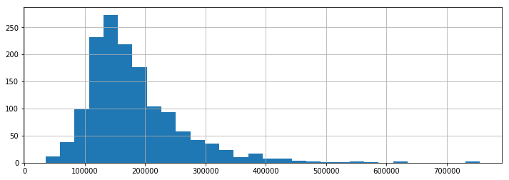
Features Correlated with SalePrice
In building regression models, correlation can help point one in the right direction of features of importance. In this set, OverallQual, GrLivArea, FullBath, GarageArea, and several other features have a positive correlation. At this point the data is not fully transformed so this remains a first-pass observation to give me a preview of what is to come.
train = ames.copy().iloc[0:1460]
test  = ames.copy().iloc[1461:]
correlated = train.corr()

plt.xticks(rotation=70)
corr_plot = correlated[1:-1].SalePrice.sort_values(ascending=False)
sns.barplot(x = corr_plot.index, y=corr_plot.values)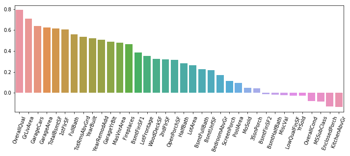
Below I’ve plotted a sample of different variable against the target variable to investigate how they’re related. While not all the plots are shown, I’ve included plots for the SaleType and Neighborhood categorical varable vs. SalePrice:
plt.xticks(rotation=45)
order = train.groupby(
        by=["SaleType"])["SalePrice"].median().sort_values().iloc[::-1]
sns.boxplot(data=train, x='SaleType', y='SalePrice',
            order = order.index.tolist())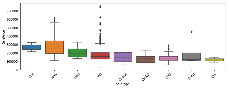
It appears that the SaleType Con (Contract 15% Down payment regular terms) yields the highest median sales price.
plt.xticks(rotation=45)
order = train.groupby(
        by=["Neighborhood"])["SalePrice"].median().sort_values().iloc[::-1]
sns.boxplot(data=train, x='Neighborhood', y='SalePrice',
            order = order.index.tolist())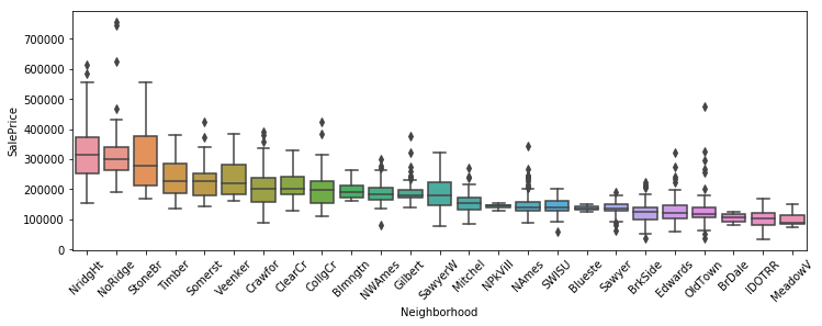
Outliers
EDA has revealed a few outliers that may hinder modelling including houses with large living areas and above-normal selling prices (See the Data Cleanup section for the code used to handle them).
sns.scatterplot(data = train, x = 'GrLivArea', y = 'SalePrice')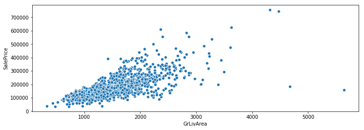
Missing Data Review
While this data contains a number of missing values, many of them aren’t true NaNs. E.g. Houses that have NaN for PoolQC or FireplaceQu are just houses that do no have pools or fireplaces, respectively. Below I review the nulls in the data set using my null_checker function (output not shown to keep it neat) and then plot the NaN counts by feature name.
ames_missing = ames[ames.columns[1:-1]].isnull().sum()
ames_missing[ames_missing>0].sort_values(ascending =False)

def null_checker(df):
    """For reviewing columns of df for completion and NaNs."""
    print("Complete columns:")
    print(str(df.columns[df.notnull().sum()==len(df)].tolist()))
    print("\n")
    for i in df.columns:
        if df[i].isnull().sum()>0:
            print("Name: " + str(i))
            print("Null Count: " + str(df[i].isnull().sum()))
            print("Null Percent: "+\
                  str(np.round((df[i].isnull().sum()/len(df[i]))*100,2))+\
                  "%")
            if df[i].dtype == 'O':
                print(str(pd.Series(df[i].value_counts().keys().tolist(),
                          index =df[i].value_counts().values.tolist())))
            else:
                print("dtype:" + str(df[i].dtype))
            print("\n")

# null_checker(ames[ames.columns[1:-1]]) # drop Id and SalesPrice columns

# Nulls summary
nulls = round(train.isnull().sum().sort_values(
        ascending=False)/len(train)*100,2)
d_types = []
for i in nulls.index:
    d_types.append(ames[i].dtype)

nulls_su = pd.DataFrame({"ColName":nulls.index,
                         "PercMissing":nulls.values,
                         "DataType":d_types})
nulls_su = nulls_su[nulls_su.PercMissing>0]

# Plot NaNs
plt.xticks(rotation=45)
sns.barplot(data=nulls_su,  x='ColName', y='PercMissing')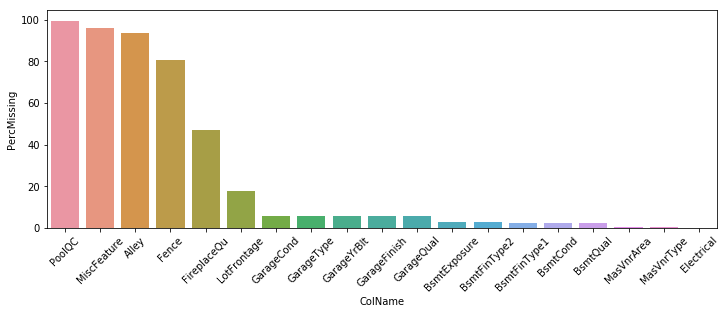
Data Cleanup & Preperation
Outliers
There are only handful of observations that contain the outliers identified through EDA. As the methods for modeling that I am using is very sensitive to outliers I will drop them.
train = train.drop(train[
        (train['GrLivArea']>4000) & (train['SalePrice']<300000)].index)

test['SalePrice'] = np.nan
ames = train.copy().append(test.copy())
Imputation
In order to use sklearn and to retain the predictive value of the variables containing numerous missing values, I need to do some targeted imputation. The below code chunk contains the transformations for this task.
# Cols to replace Pools, Alleys, Fences, Fireplaces, and Misc feats w/ "none"
none_cols = nulls_su[nulls_su.PercMissing > 20].ColName.tolist()
for i in none_cols:
    ames[i] = ames[i].fillna("None")

# use the lot frontage median by neighborhood to fill in lot frontage NaNs.
ames["LotFrontage"] = ames.groupby(
        "Neighborhood")["LotFrontage"].transform(lambda x: x.fillna(x.median()))

# Garages NaNs
for i in ['GarageCond', 'GarageType', 'GarageFinish', 'GarageQual']:
    ames[i] = ames[i].fillna("None")

for i in ['GarageYrBlt', 'GarageArea', 'GarageCars']:
    ames[i] = ames[i].fillna(0)

# Basement NaNs
for i in ['BsmtQual', 'BsmtCond', 'BsmtExposure', 'BsmtFinType1',
          'BsmtFinType2']:
    ames[i] = ames[i].fillna("None")

for i in ['BsmtFinSF1', 'BsmtFinSF2', 'BsmtUnfSF','TotalBsmtSF',
          'BsmtFullBath', 'BsmtHalfBath']:
    ames[i] = ames[i].fillna(0)

# Vaneer Types and MSZoning
ames["MasVnrType"] = ames["MasVnrType"].fillna("None")
ames["MasVnrArea"] = ames["MasVnrArea"].fillna(0)
ames['MSZoning'] = ames['MSZoning'].fillna(ames['MSZoning'].mode()[0])

# Deal with 1-off missing values
ames = ames.drop(['Utilities'], axis=1) # only in training data
ames["Functional"] = ames["Functional"].fillna("Typ") # most common
ames["Electrical"] = ames['Electrical'].fillna(ames['Electrical'].mode()[0])
ames['KitchenQual'] = ames['KitchenQual'].fillna(ames['KitchenQual'].mode()[0])

# Last few NaNs
for i in ['Exterior1st', 'Exterior2nd', 'SaleType']:
    ames[i] = ames['Exterior2nd'].fillna(ames['Exterior2nd'].mode()[0])

null_checker(ames)
Complete columns:
['Id', 'MSSubClass', 'MSZoning', 'LotFrontage', 'LotArea', 'Street', 'Alley',
'LotShape', 'LandContour', 'LotConfig', 'LandSlope', 'Neighborhood', 'Condition1',
'Condition2', 'BldgType', 'HouseStyle', 'OverallQual', 'OverallCond', 'YearBuilt',
'YearRemodAdd', 'RoofStyle', 'RoofMatl', 'Exterior1st', 'Exterior2nd', 'MasVnrType',
'MasVnrArea', 'ExterQual', 'ExterCond', 'Foundation', 'BsmtQual', 'BsmtCond',
'BsmtExposure', 'BsmtFinType1', 'BsmtFinSF1', 'BsmtFinType2', 'BsmtFinSF2', 'BsmtUnfSF',
'TotalBsmtSF', 'Heating', 'HeatingQC', 'CentralAir', 'Electrical',
'1stFlrSF', '2ndFlrSF', 'LowQualFinSF', 'GrLivArea', 'BsmtFullBath', 'BsmtHalfBath',
'FullBath', 'HalfBath', 'BedroomAbvGr', 'KitchenAbvGr', 'KitchenQual', 'TotRmsAbvGrd',
'Functional', 'Fireplaces', 'FireplaceQu', 'GarageType', 'GarageYrBlt', 'GarageFinish',
'GarageCars', 'GarageArea', 'GarageQual', 'GarageCond', 'PavedDrive', 'WoodDeckSF',
'OpenPorchSF', 'EnclosedPorch', '3SsnPorch', 'ScreenPorch', 'PoolArea', 'PoolQC',
'Fence', 'MiscFeature', 'MiscVal', 'MoSold', 'YrSold', 'SaleType', 'SaleCondition']
Name: SalePrice
Null Count: 1458
Null Percent: 50.0%
dtype:float64
Above, the null_checker function indicates that only the test portion of the data still contains missing values which is expected from the kaggle data.
Ordinal Categorical Variables
Many of the features that end in Qu or QC represent a quality score from low to high. Below I use sklearns LabelEncoder object to transform these ordinal categorical variables to numeric representations.
ordinals = ['FireplaceQu', 'BsmtQual', 'BsmtCond', 'GarageQual', 'GarageCond',
            'ExterQual', 'ExterCond','HeatingQC', 'PoolQC', 'KitchenQual',
            'BsmtFinType1', 'BsmtFinType2', 'Functional', 'Fence',
            'BsmtExposure', 'GarageFinish', 'LandSlope', 'LotShape',
            'PavedDrive', 'Street', 'Alley', 'CentralAir', 'MSSubClass',
            'OverallCond', 'YrSold', 'MoSold']
for i in ordinals:
    lbl = LabelEncoder()
    lbl.fit(list(ames[i].values))
    ames[i] = lbl.transform(list(ames[i].values))

ames[ordinals].iloc[:,0:6].head()| FireplaceQu | BsmtQual | BsmtCond | GarageQual | GarageCond | ExterQual | |
|---|---|---|---|---|---|---|
| 0 | 3 | 2 | 4 | 5 | 5 | 2 |
| 1 | 5 | 2 | 4 | 5 | 5 | 3 |
| 2 | 5 | 2 | 4 | 5 | 5 | 2 |
| 3 | 2 | 4 | 1 | 5 | 5 | 3 |
| 4 | 5 | 2 | 4 | 5 | 5 | 2 |
Feature Engineering
Below I’ll add one additional feature for improving the prediction called TotalSF that contains the total square footage of existing variables.
Following that I will complete a log transformation on the target variable and set it aside in y_train, update the train and test variables, record the Ids of each, and drop non-feature columns.
ames['TotalSF'] = ames['TotalBsmtSF'] + ames['1stFlrSF'] + ames['2ndFlrSF']

train = ames.copy()[ames.Id <= 1460]
y_train = np.log1p(train.SalePrice)
test  = ames.copy()[ames.Id > 1460] #

train_ID = train['Id']
test_ID = test['Id']

train.drop(['Id', 'SalePrice'], axis=1, inplace=True)
test.drop(['Id', 'SalePrice'], axis=1, inplace=True)

ames = train.copy().append(test.copy())
Power Transformation
A few of the variables in the data contain high levels of skew that can cause problems with model training. Fortunatley, a Box Cox transformations can reduce the skew and help normalize values to make them more amenable to fitting.
num_feats = ames.dtypes[ames.dtypes != "object"].index
skew_feats = ames[num_feats].apply(
        lambda x: skew(x.dropna())).sort_values(ascending=False)

skew_df = pd.DataFrame({'Skew' :np.abs(skew_feats)})
Numeric Variables as Categories & Dummy Variables
Features such as MSSubClass, OverallCond, YrSold, and MoSold are numerically represented but are actually categorical and therefore need to be updated to objects. Creating dummy variables of categorical features can improve model performance at the cost of requiring many more features. While this data set is complex, the number of columns is not absolutely massive so we can use dummy variables without much performance loss:
# Changing to strings as categorical
ames['MSSubClass'] = ames['MSSubClass'].apply(str)
for i in ['OverallCond', 'YrSold', 'MoSold']:
    ames[i] = ames[i].astype(str)
# ames.shape # (2916, 79)

# Dummify Categorical
ames_new = pd.get_dummies(ames)

train = ames_new.copy().iloc[0:len(y_train)]
test  = ames_new.copy().iloc[(len(y_train)):]

ames.describe(include='object').iloc[:,0:5]| MSSubClass | MSZoning | LandContour | LotConfig | Neighborhood | |
|---|---|---|---|---|---|
| count | 2916 | 2916 | 2916 | 2916 | 2916 |
| unique | 16 | 5 | 4 | 5 | 25 |
| top | 0 | RL | Lvl | Inside | NAmes |
| freq | 1078 | 2267 | 2621 | 2131 | 442 |
Model Creation and Validation
To keep things digestible, I am going to create and compare only two different models: A linear regression Lasso model and an ensemble GradientBostingRegressor model.
Cross Validation Function
def cv_rmsle(model, n_folds = 10):
    """Cross validation using n_folds"""
    kf = KFold(n_folds,
               shuffle=True,
               random_state=42
               ).get_n_splits(train.values)

    rmse = np.sqrt(-cross_val_score(model,
                                    train.values,
                                    y_train,
                                    scoring="neg_mean_squared_error", cv = kf))
    return(rmse)
Models
Below I employ the make_pipeline object to impliment the RobustScaler() prior to fitting the Lasso model. Using the RobustScaler() reduces the impact of outliers when fitting the Lasso model, which is sensitive to outliers. For the GradientBoostingRegressor model, I employ the huber loss function that makes the fit less sensitive to outliers:
m_lasso = make_pipeline(RobustScaler(),
                        Lasso(alpha =0.0005,
                              random_state=1))

m_GBoost = GradientBoostingRegressor(n_estimators = 3000,
                                     learning_rate = 0.05,
                                     max_depth = 4,
                                     max_features = 'sqrt',
                                     min_samples_leaf = 15,
                                     min_samples_split = 10,
                                     loss='huber',
                                     random_state = 5)
Preliminary Model Fit & Scoring
%time scores_lasso = cv_rmsle(m_lasso)Wall time: 3.93 s%time scores_GBoost = cv_rmsle(m_GBoost)Wall time: 2min 12sBelow, the model’s average RSMLE scores are similar across the 10 runs. However, the time to run m_lasso was much faster at approx 4 seconds than m_GBoost that took over 2 minutes. Time to fit is an important consideration given that compute-time can be costly.
print("Lasso Model RSME: mean: {:.3f}, std: {:.3f}\n".format(scores_lasso.mean(),
                                                        scores_lasso.std()))
print("GBoost Model RSME: mean: {:.3f}, std: {:.3f}".format(scores_GBoost.mean(),
                                                         scores_GBoost.std()))
Lasso Model RSME: mean: 0.112, std: 0.013
GBoost Model RSME: mean: 0.117, std: 0.015Following 10 seperate model fits and scores, the m_lasso regression model appears to have slightly better predictive power than the m_GBoost model. That seems ok given that the m_lasso model is so much faster to run and fit.
Given that the error was cacluated on the transformed target variable, it’s wise to get a little more clarity on the actual predictive power of each model by measuring the error on the inverse transformed values. Below we create a predictions data frame that contains these values.
m_GBoost.fit(train, y_train)                           # Fit the models
m_lasso.fit(train, y_train)

train_true = np.expm1(y_train)                         # return log-transformed $'s to $'s

Boost_train_pred = m_GBoost.predict(train)             # return predicted log-transformed to $'s
Boost_train_pred_revert  = np.expm1(Boost_train_pred)

Lasso_train_pred = m_lasso.predict(train)
Lasso_train_pred_revert  = np.expm1(Lasso_train_pred)

predictions = pd.DataFrame({"Id":train_ID,             # Combine results in a df
                            "True Values":train_true,
                            "Lasso_SP":np.round(Lasso_train_pred_revert),
                            "Boost_SP":np.round(Boost_train_pred_revert)})
predictions = predictions.assign(LassoDelta = predictions['True Values']- predictions.Lasso_SP)
predictions = predictions.assign(GBoostDelta = predictions['True Values']- predictions.Boost_SP)
Below I measure the Mean Absolute Error (MAE) on the inverse-transformed predictions vs the true predictions. This will provide the error in absolute dollars:
lasso_MAE  = mean_absolute_error(predictions['True Values'], predictions['Lasso_SP'])
GBoost_MAE = mean_absolute_error(predictions['True Values'], predictions['Boost_SP'])

print("Lasso Model MAE: mean: {:.2f}\n".format(lasso_MAE))
print("GBoost Model MAE: mean: {:.2f}".format(GBoost_MAE))
Lasso Model MAE: mean: 12405.70
GBoost Model MAE: mean: 3151.58While m_lasso and m_GBoost models may have performed similarly across the 10 runs of the cross validation, the inverse transformed error values of the MAE make the m_GBoost model the clear winner. m_lasso makes predictions with errors that are 4 times greater than m_GBoost on average across the training set.
A random sample of the predictions in dollars along with deltas from the true values illustrate this further. As shown in the table below the deltas are smaller within the GBoostDelta column than the LassoDelta column.
predictions.sample(n = 10, random_state = 2)| Id | True Values | Lasso_SP | Boost_SP | LassoDelta | GBoostDelta | |
|---|---|---|---|---|---|---|
| 239 | 240 | 113000.0 | 125163.0 | 115439.0 | -12163.0 | -2439.0 |
| 961 | 962 | 272000.0 | 286988.0 | 270498.0 | -14988.0 | 1502.0 |
| 960 | 961 | 116500.0 | 121616.0 | 117324.0 | -5116.0 | -824.0 |
| 602 | 603 | 220000.0 | 221415.0 | 215211.0 | -1415.0 | 4789.0 |
| 308 | 309 | 82500.0 | 98999.0 | 95016.0 | -16499.0 | -12516.0 |
| 173 | 174 | 163000.0 | 157004.0 | 158844.0 | 5996.0 | 4156.0 |
| 1217 | 1218 | 229456.0 | 234217.0 | 237389.0 | -4761.0 | -7933.0 |
| 679 | 680 | 128500.0 | 125809.0 | 128493.0 | 2691.0 | 7.0 |
| 226 | 227 | 290000.0 | 254979.0 | 282024.0 | 35021.0 | 7976.0 |
| 349 | 350 | 437154.0 | 457661.0 | 437840.0 | -20507.0 | -686.0 |
Closing Remarks
This post provided a simplified walk through of a bottoms-up EDA, model development, prediction, and model evaluation of the Ames data using two different regression methods. While the models created provide decent results, this post is only meant to be a digestible example of my regression work and an example of the sklearn library in action. There are numerous model configurations and types that have not been investigated including hybrid models but for now we’ll leave that for future posts!